Seismic impedance and reflection: a worked example
Worked seismic examples: calculate reflection coefficients, compare bed resolution, understand sampling aliasing, and interpret reflection terminations.
Start with a property contrast, not a rock-name guess
Acoustic impedance is density multiplied by P-wave velocity. A reflector marks a contrast in that product. Different rock and fluid combinations can share an impedance, so a bright event alone does not identify a formation or prove hydrocarbons. Geological context and well ties help constrain the alternatives.
A two-layer calculation you can reproduce
This invented example uses homogeneous, lossless layers and a plane P wave at normal incidence. The angle is zero from the interface normal, not from the bedding plane. We use pressure amplitudes and number layers in the direction of the incident wave.
Teaching values, not measurements
Layer
Density, kg/m³
P velocity, m/s
Impedance, kg/(m²·s)
1, upper
2,000
3,000
6,000,000
2, lower
2,500
3,600
9,000,000
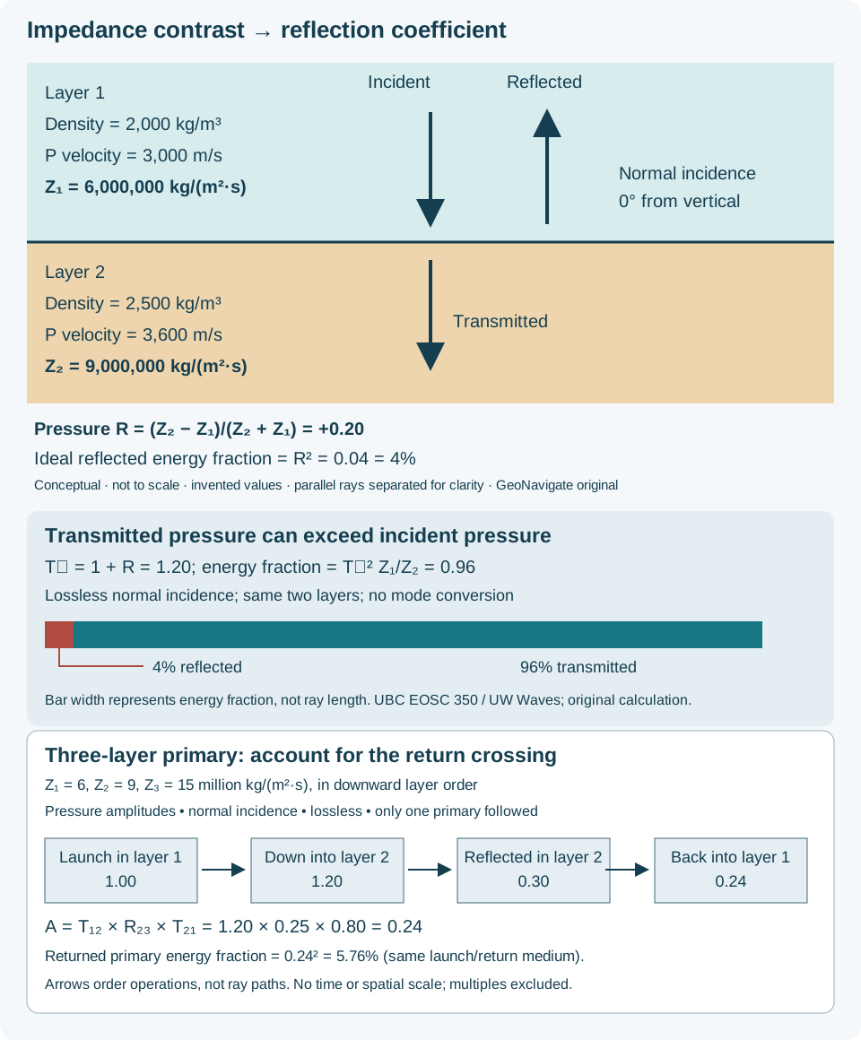
The reflection coefficient is R = (Z₂ − Z₁)/(Z₂ + Z₁) = (9 − 6)/(9 + 6) = +0.20. The common factor of one million cancels. For a unit incident pressure amplitude, the reflected pressure amplitude is +0.20 at the interface. In this ideal case, the reflected energy fraction is R² = 0.04, or 4%, not 20%.
Reverse the contrast, then test your interpretation
Keep the incident-side impedance at 6 million but change the lower value to 3 million. R becomes (3 − 6)/(3 + 6) = −1/3. The reflected pressure pulse reverses sign relative to the incident pulse. Setting both impedances to 6 million instead gives zero in this ideal model, even if the two layers have different density and velocity combinations. These tests are useful checks on a spreadsheet formula and its layer ordering.
Why a seismic trace is not a coefficient list
A reflectivity series locates interface coefficients in travel time. Each coefficient scales a time-shifted wavelet; their sum forms a simple synthetic trace. Overlapping pulses alter the resulting appearance. Acquisition, processing and phase conventions also affect the display, so “positive coefficient” should not be equated with a particular black peak without checking the convention.
Keep time and depth separate
For an invented 300 m thick upper layer at 3,000 m/s and a vertical down-and-back path, two-way time is 2 × 300 / 3,000 = 0.20 s. This is a time coordinate, not 200 m of depth. A layered depth conversion requires the appropriate velocities and path geometry. Dipping structures and nonzero offsets require more than this vertical example. Work through a two-layer depth conversion and velocity sensitivity below.
A practical review sequence
Record density and velocity units, source interval and data quality before multiplying.
Identify the incident side and state the amplitude/sign convention.
Check equal-impedance and reversed-contrast cases to catch formula errors.
Compare a synthetic trace with the field trace using a documented wavelet and time-depth tie.
Retain alternatives where lithology, fluids, resolution or data processing could explain the same response.
A deeper primary reflection crosses the upper boundary twice
A reflectivity series is useful input to a simple convolution model. UBC notes that actual event amplitudes are also modified by transmission coefficients. The following original calculation isolates that effect; it does not simulate a complete seismic record.
Worked three-layer pressure-amplitude ledger
Take horizontal, homogeneous, lossless layers with acoustic impedances Z₁ = 6, Z₂ = 9 and Z₃ = 15 million kg/(m²·s), increasing downward. Launch a unit plane-wave pressure amplitude downward in layer 1 at normal incidence. Follow only the primary reflected from the layer 2–3 boundary and returned into layer 1:
Returned primary amplitude in layer 1: A = 1.20 × 0.25 × 0.80 = 0.24, relative to the original incident pressure amplitude.
Using 0.25 alone overstates this model's returned primary. The two upper-boundary transmissions multiply to 0.96 = 1 − R₁₂², where R₁₂ = 0.20. This 0.96 is an amplitude multiplier for the round trip, not the returned primary's energy fraction. Since launch and return are in the same medium, that isolated primary has energy-flux fraction 0.24² = 0.0576, or 5.76%.
Original conceptual diagram, not to spatial scale. The bottom ledger orders amplitude operations; arrows are not ray paths. Enlarge the SVG.
This calculation omits spreading, attenuation, source and receiver responses, the shallow reflected event and all multiples. No layer thickness or velocity is specified, so no arrival time follows. For a timed synthetic, add a consistent velocity–thickness model and wavelet. Compare single-interface energy balance and the oilfield reflectivity entry.
Counterexample: different properties, no impedance contrast
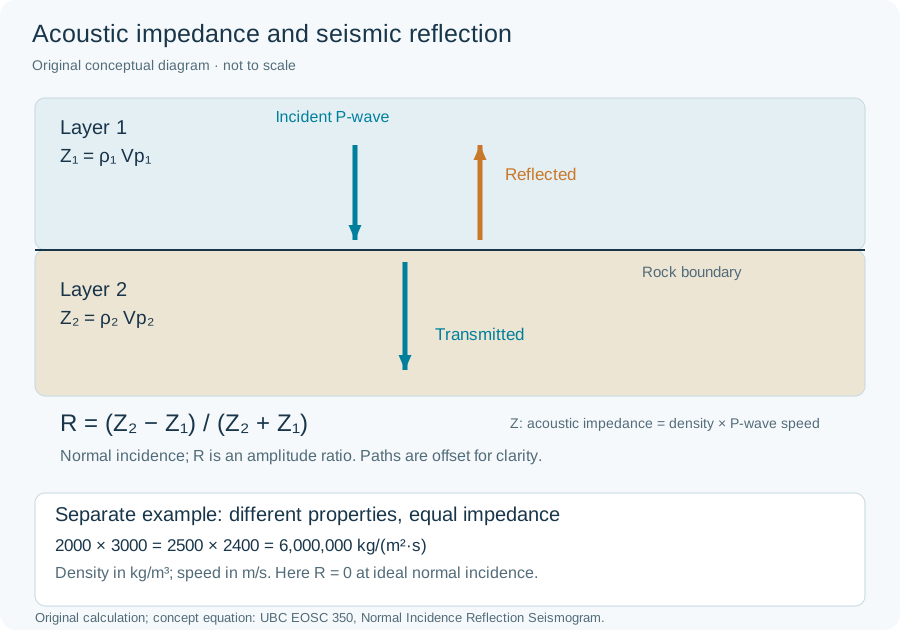
For two hypothetical layers, ρ₁ = 2000 kg/m³ and Vp₁ = 3000 m/s give Z₁ = 6,000,000 kg/(m²·s). Set ρ₂ = 2500 kg/m³ and Vp₂ = 2400 m/s: Z₂ is identical, so R = (Z₂ − Z₁)/(Z₂ + Z₁) = 0. Density increased while speed decreased. The lower panel of the shared impedance schematic records this separate case.
This ideal normal-incidence result does not prove identical lithology or predict an oblique-incidence response. Keep density, velocity and impedance distinct when tying wells to seismic. Equation context: UBC EOSC 350; original illustrative inputs, not measured rocks.
Original conceptual schematic, not to scale. Upper arrows describe a general interface; the separate lower calculation has R = 0. Open full-size. Concept reference: UBC EOSC 350 above.
Seismic wavelength, bed separability and sampling
A reflector’s visibility and the separation of its top and base answer different questions. Vertical seismic resolution concerns that separation. A thin bed may change a trace without producing two independently interpretable boundary events. Seismic tuning can change both amplitude and apparent event shape.
Worked frequency comparison
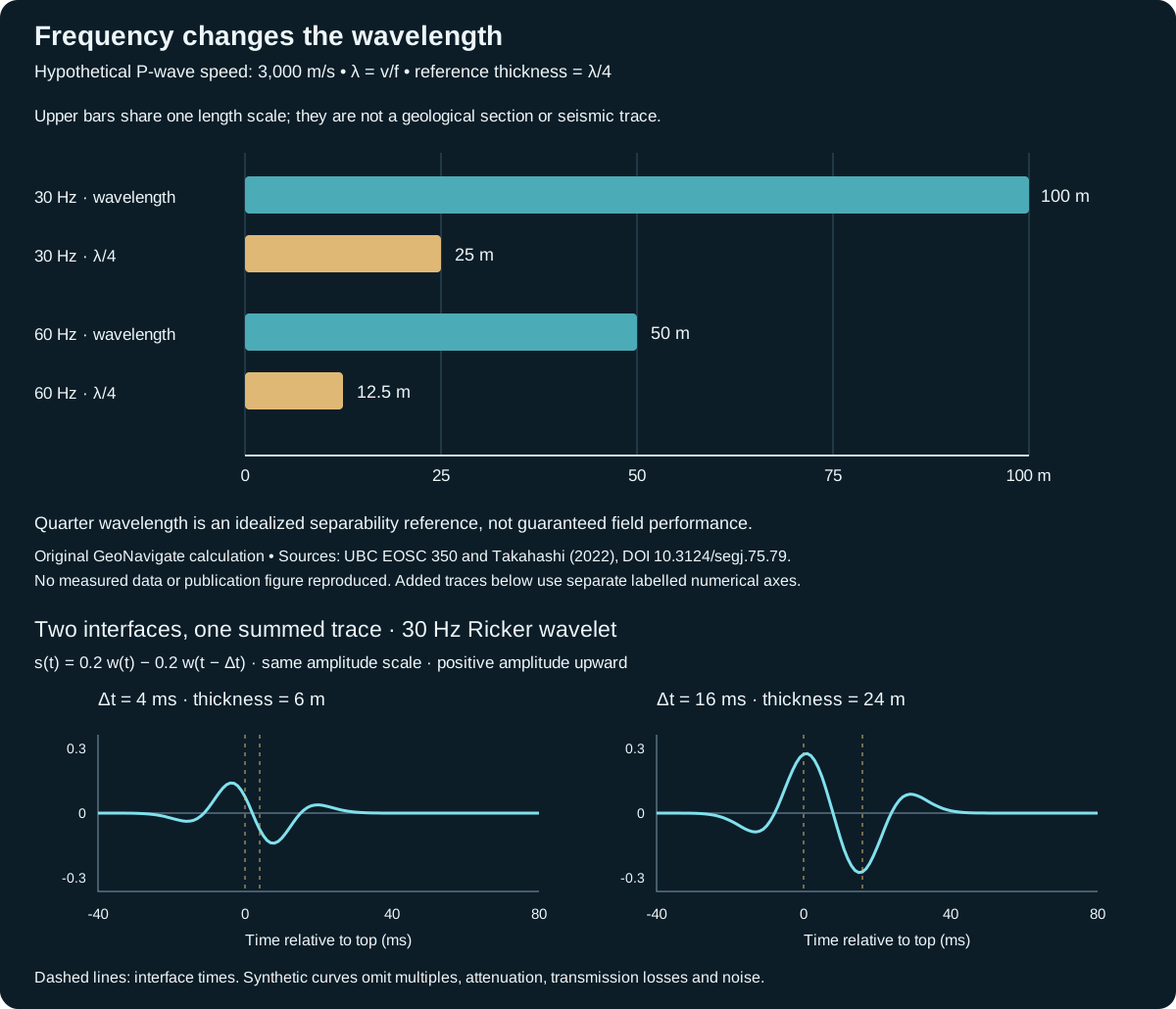
Assume a homogeneous target layer with invented P-wave velocity 3,000 m/s, horizontal boundaries and vertical propagation. Use two illustrative target frequencies, 30 and 60 Hz. From λ = v/f, the corresponding wavelengths are 100 and 50 m. Applying the same quarter-wavelength convention gives reference thicknesses of 25 and 12.5 m. These are estimates under a stated criterion, rather than survey acceptance thresholds.
Hypothetical comparison at constant velocity
Frequency
Wavelength
λ/4
Top-to-base two-way separation at λ/4
30 Hz
100 m
25 m
16.67 ms
60 Hz
50 m
12.5 m
8.33 ms
Original GeoNavigate calculation; invented values. Bars use the labelled length scale. They are not bed geometry or computed waveforms. Open full-size SVG.
Check the time conversion
For the 25 m reference thickness, the extra down-and-back travel time is 2 × 25 / 3,000 = 0.01667 s. The 12.5 m case gives 0.00833 s. If the recording interval were 2 ms, its nominal depth increment under this same velocity assumption would be 3 m. That increment tells you where samples are stored; it does not establish that two boundaries 3 m apart can be resolved. Interpolation can create additional plotted samples without adding independent observations.
Worked example: sum the reflections before picking a bed
Keep velocity at 3,000 m/s and use the invented zero-phase Ricker wavelet w(t) = [1 − 2(πft)²] exp[−(πft)²], with spectral peak frequency f = 30 Hz and t in seconds. Place a +0.2 reflection at t = 0 and a −0.2 reflection at t = Δt. In a simple convolution model, the combined response is s(t) = 0.2 w(t) − 0.2 w(t − Δt). These are prescribed coefficients; the exercise omits transmission losses, multiples, attenuation and noise.
The added panels above calculate this sum at 1 ms intervals, joining samples for display. A separation of 4 ms represents thickness vΔt/2 = 6 m; 16 ms represents 24 m. Both panels use identical frequency and amplitude scales. Only the boundary spacing changes. The dashed lines locate the model interfaces; they are not picks made from the resulting extrema.
As a check, at Δt = 0 the two opposite coefficients cancel exactly in this model. At finite separation, overlapping wavelet lobes change the trace shape and amplitude. Picking its strongest positive and negative extrema need not recover the prescribed interface times. This is why detection of a thin interval and independent picking of its two boundaries are different interpretation tasks.
The plotted 1 ms interval is a numerical display choice, not a claim of 1.5 m geological resolution. Changing the wavelet, phase or coefficient signs would change the response. Before using this logic on a well tie, document the target wavelet, time-depth relationship and processing conventions; retain thickness alternatives that produce similar responses.
Estimate the wavelet and useful frequency band at the target, with an appropriate interval velocity. Higher-frequency energy can weaken with propagation; a source specification alone is insufficient.
State whether the question is detection, boundary separation or thickness estimation. Amplitude-based inference needs its own assumptions and uncertainty assessment.
Compare seismic, logs and core at compatible scales. Preserve unresolved alternatives when a thin interval affects the trace but its boundaries cannot be picked separately.
Sampling aliasing: two signals, identical recorded points
A densely drawn seismic trace may contain many interpolated display points. To assess sampling aliasing, inspect the original sample interval and acquisition filters. A smooth display alone cannot establish that the underlying signal was adequately sampled.
Worked example with invented cosine signals
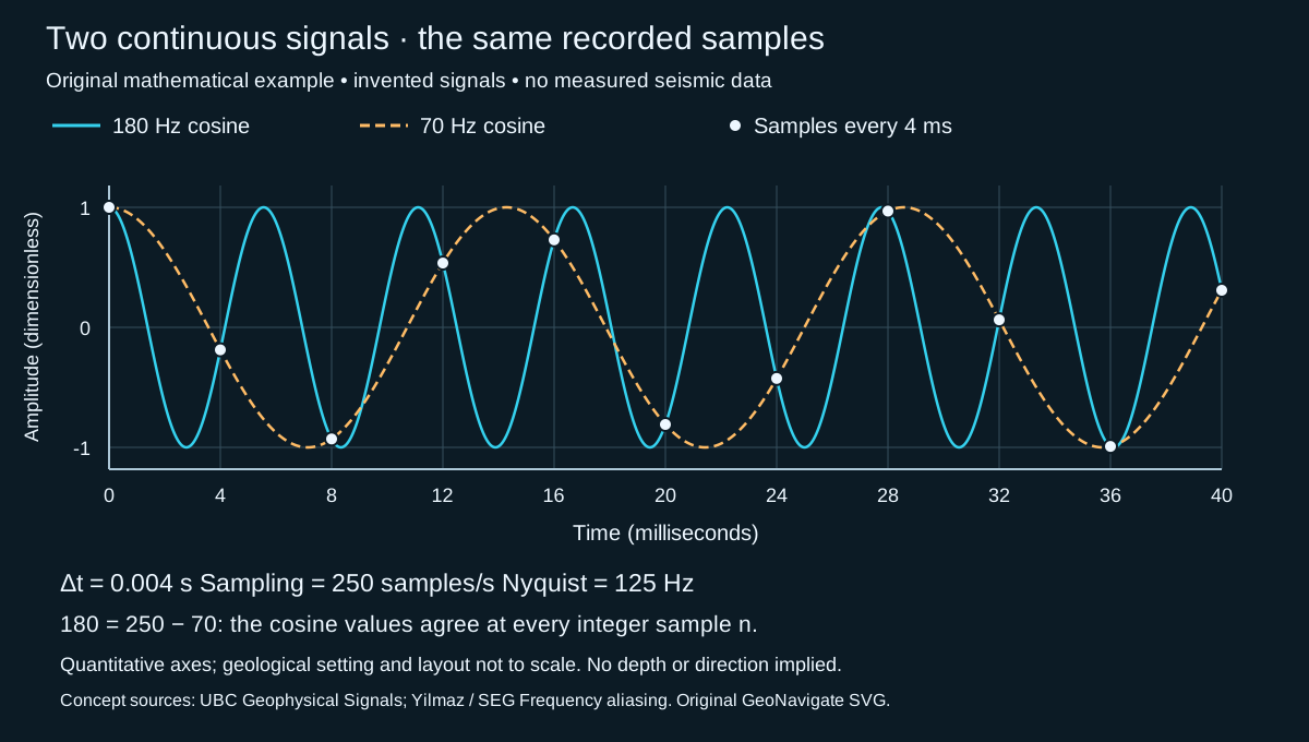
Choose a uniform interval Δt = 4 ms = 0.004 s. The sampling frequency is 1/0.004 = 250 samples/s; the Nyquist frequency is half that, 125 Hz. Consider unit-amplitude signals A(t) = cos(2π × 180t) and B(t) = cos(2π × 70t), with t in seconds and the same time origin.
Original mathematical example with invented signals; not a measured trace or an author's published figure. Axes are quantitative; geological setting and page layout are not to scale. No depth or compass direction is implied. Open full-size SVG.
At sample n, t = n/250 s. Because 180 = 250 − 70, A(n/250) = cos(2πn − 2π × 70n/250) = B(n/250). The equality holds for every integer n, not only the eleven plotted points. At 4 ms both values are about −0.1874; at 8 ms both are about −0.9298. Between samples the curves differ. The 180 Hz signal lies above Nyquist and shares these samples with a 70 Hz signal below it.
Change the acquisition, then check the assumptions
If the interval were 2 ms, the sample frequency would be 500 samples/s and Nyquist would be 250 Hz. Our two stipulated frequencies would both fall below that boundary. At the new 2 ms sample, A is about −0.6374 and B about +0.6374: they are distinguishable. This comparison assumes noiseless, point samples of only the stated signals. It is not a recommended field recording specification.
Equality with the boundary is unsafe for an arbitrary phase. At 4 ms intervals, sin(2π × 125t) is zero at every sample. Knowing only those zeros would not reveal its amplitude. Real acquisition therefore needs a retained band below Nyquist and suitable anti-alias filtering before sampling; downsampling also needs filtering before points are discarded. Filtering an already aliased record cannot uniquely untangle components that have become indistinguishable.
Connect sampling to geological interpretation
Time sampling and vertical seismic resolution answer different questions. The 125 Hz boundary above gives no target velocity, wavelet, noise level or bed thickness. Do not substitute it for the useful target frequency in a wavelength calculation.
Spatial sampling needs its own review: a fine time interval cannot repair coarse receiver or trace spacing. A regularly sampled spatial sinusoid has a corresponding limit of 1/(2Δx) cycles per metre when Δx is in metres. Apparent arrivals can become directionally ambiguous when spatial sampling is inadequate. Survey geometry, wavefield complexity and migration matter; the time-series calculation here is not a spatial reconstruction algorithm.
Reflection terminations: name the geometry before the history
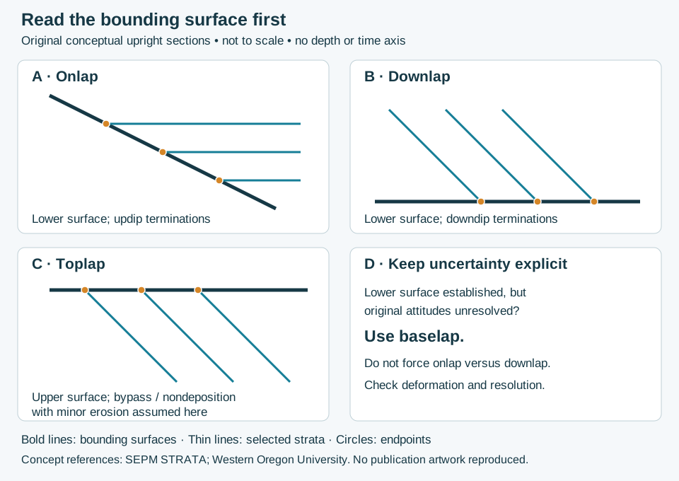
Start by identifying the package and its bounding surface. Onlap and downlap meet a lower surface; toplap meets an upper surface. The distinction is relative to the package, not simply the top or bottom of the screen. Baselap preserves a lower-termination observation when onlap versus downlap remains unresolved.
Original GeoNavigate conceptual geometry, not to scale. Thin lines are selected strata, not simulated seismic amplitudes. No numerical dip, geographic direction, depth or travel-time coordinate is assigned. Open full-size SVG.
Worked interpretation: three sketches, three evidence statements
Panel A: the horizontal lines lie above the sloping lower surface and end against it toward the left, progressively up that surface. In this stipulated undeformed geometry, identify onlap.
Panel B: inclined lines lie above the lower surface and end toward their downdip side, to the right. Identify downlap. Do not label the surface a maximum flooding surface solely from this drawing.
Panel C: inclined lines end beneath an upper surface. The stated model assumes bypass or nondeposition with only minor erosion, supporting toplap. If independent evidence instead showed substantial removal, describe erosional truncation; the line pattern alone does not measure erosion.
Change the evidence: deformation obscures the original geometry
Suppose a folded section preserves a lower contact and three endpoints, but restoration is uncertain. Keep the observation as baselap and record the unresolved original attitudes. A confident lower-contact pick and an uncertain depositional interpretation can coexist. Rotating a screenshot is not a structural restoration. Check younging, fault repetition and section orientation before using present-day angles as depositional slopes.
From an ideal section to seismic and well data
The sketches contain exact endpoints by construction. Real reflections can lose continuity where signal quality, interference or resolution changes. Review neighbouring traces and intersecting lines before treating a fading event as a geological termination. Compare the resolution discussion and the sampling example above. A time-section slope is not a measured bed dip in depth.
At a well tie, retain the documented time–depth relationship and check sample/log depth references. A missing log motif could represent erosion, nondeposition, a facies change, incomplete coverage or structural omission. One well does not determine the lateral termination geometry. Record the alternatives and the evidence needed to reject them rather than forcing the well into a preferred sequence model.
Time to depth: choose the velocity and datum before the arithmetic
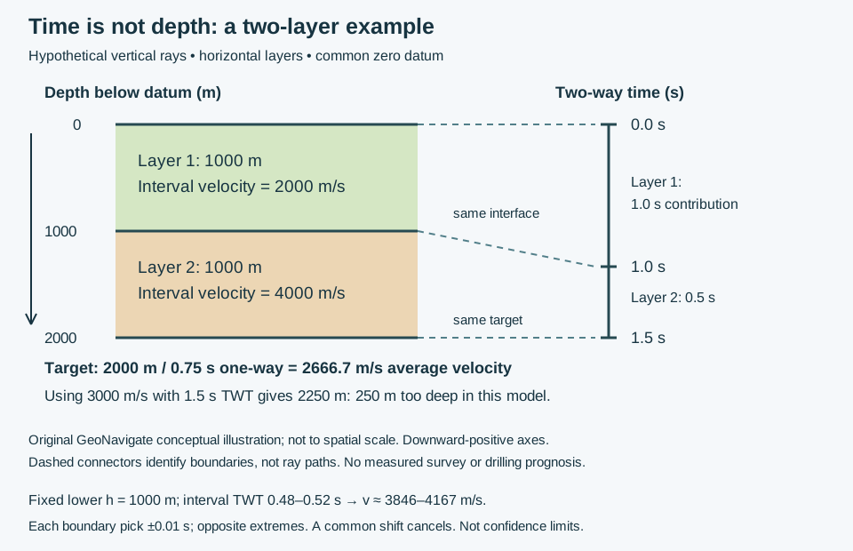
A seismic image may resemble a cross-section while its vertical coordinate is two-way travel time (TWT). Depth conversion needs a velocity model. In a horizontal layer traversed vertically, the two-way contribution is Δt = 2h/v. Add layer times before calculating average seismic velocity to a target. This is an ideal model, not a universal conversion of events on an unmigrated section.
Original GeoNavigate hypothetical model, not to spatial scale. Depth and time increase downward from a common datum. Dashed connectors identify boundaries, not rays. Open full-size SVG.
Worked example: two equal-thickness layers
Assume a 1000 m upper layer at 2000 m/s and a 1000 m lower layer at 4000 m/s. These are interval velocities. Source and receiver coincide at the zero reference surface; the target is horizontal, 2000 m below it. Ignore lateral variation and anisotropy.
Average velocity: 2000 / 0.75 ≈ 2666.7 m/s. Recover depth with 2666.7 × 1.50 / 2 ≈ 2000 m.
The arithmetic mean of the two velocities is 3000 m/s. Applying it to 1.50 s gives 2250 m, 250 m too deep in this model. Equal thicknesses do not mean equal travel-time weights. Applying the lower velocity, 4000 m/s, to the entire time column is also wrong: that velocity belongs to the lower 0.50 s contribution.
Sensitivity is not a confidence interval
At a fixed TWT of 1.50 s, assumed average velocities of 2500 and 2800 m/s give depths of 1875 and 2100 m. That 225 m spread is a chosen scenario range, not a probabilistic uncertainty estimate. At a fixed 2666.7 m/s, a ±10 ms change in picked TWT changes depth by approximately ±13.3 m. Velocity, event-identification, timing and datum errors may coexist; these separate calculations do not describe their combined distribution.
Two boundary picks: test the difference
Keep the lower-layer thickness fixed at 1000 m. Allow each cumulative TWT pick, 1.00 s and 1.50 s, to vary by ±0.01 s. Opposite extreme shifts give interval times from 1.49 − 1.01 = 0.48 s to 1.51 − 0.99 = 0.52 s. Thus v = 2h/Δt ranges from about 3846 to 4167 m/s. This is a bounded sensitivity exercise, not a confidence interval. If both picks instead share exactly the same timing shift, their difference remains 0.50 s and the calculated interval velocity stays 4000 m/s. Unknown thickness, different event picks and ray geometry introduce other errors; do not infer a velocity change from timing differences alone.
Apply the logic at the well tie
A checkshot survey records source-to-receiver arrivals at known positions. Reconcile source offset, well deviation and the seismic reference datum before comparing its time–depth curve with surface seismic. Do not simply double an uncorrected slant-path arrival. Vertical distance below datum, elevation and measured depth along the borehole are different quantities.
In a drilling discussion, a target at 1.50 s is a time pick plus a model-dependent depth estimate. Record the velocity model, datum, well control and event tie. In folded or faulted terrain, examine migration, lateral velocity changes and possible repeated sections before treating every mismatch as a depth error. No operational target or well-specific prognosis is supplied by this example.
Keep the data product explicit
A scanned section provides an image with axes and annotations to calibrate. Digitizing its horizon does not recover original numerical trace amplitudes. A numerical trace file still needs verified sample units, coordinates and processing history. Interpolating picked horizons adds a geometric model; it does not create a measured three-dimensional seismic amplitude volume. Identify the product before combining it with well data.
Transmission: why an amplitude above one does not create energy
Use the same invented two-layer model above: Z₁ = 6 million and Z₂ = 9 million kg/(m²·s), with a wave incident from layer 1. Retain the lossless plane-wave, normal-incidence assumptions and pressure-amplitude convention. Do not substitute a displacement coefficient or an energy fraction into this calculation.
Keep pressure and intensity ratios separate
The pressure reflection coefficient is R = (9 − 6)/(9 + 6) = +0.20.
Pressure continuity at the interface gives pᵢ + pᵣ = pₜ. Dividing by incident amplitude gives Tₚ = 1 + R = 1.20, equivalently 2Z₂/(Z₁ + Z₂).
The reflected energy-flux fraction is R² = 0.04, because incident and reflected waves occupy the same medium.
The transmitted fraction is Tₚ² Z₁/Z₂ = 1.20² × 6/9 = 0.96. The check is 0.04 + 0.96 = 1.
For a travelling plane wave in this model, intensity is proportional to squared pressure amplitude divided by impedance. Consequently, a larger pressure amplitude in the higher-impedance layer does not imply more transmitted energy than arrived. Squaring 1.20 alone would give 1.44 and omit the essential impedance factor. The lower panel of the shared full-size schematic shows the 4:96 energy split with proportional widths.
A reversed-direction check
Send a separate wave from the 9-million side toward the 6-million side. Now R = −0.20 and Tₚ = 0.80. The transmitted fraction is 0.80² × 9/6 = 0.96 again. The pressure reflection sign reverses and transmitted amplitude changes, while the ideal energy fractions remain the same. This is an algebra check, not a prediction of an acquired seismic trace.
Limits in geological interpretation
These fractions apply at one ideal interface. Propagation losses, geometrical spreading, multiple reflections and acquisition response affect recorded amplitudes. Oblique elastic incidence can convert wave modes and requires the appropriate coefficients; the simple formulas above are insufficient. Keep the incident side, amplitude convention and material assumptions with any exported calculation. Compare reflection coefficient, acoustic impedance and normal incidence.