Groundwater flow: head, permeability and a worked Darcy example

Worked measurement example: depth to water versus head

Separate storage, flow capacity and driving force

A porous sandstone can store water without transmitting it rapidly. Porosity describes void space; permeability describes the connected medium’s ability to transmit fluid. Hydraulic conductivity also depends on the fluid’s density and viscosity. The driving force is a difference in hydraulic head, not simply a difference in ground elevation.

Start with the definitions of hydraulic head, hydraulic gradient and hydraulic conductivity. Reservoir readers can compare the oilfield permeability terminology.

A hypothetical saturated-sandstone example

Assume steady horizontal flow through a homogeneous, isotropic segment containing water of uniform density. Two piezometers sample the same hydraulic unit, 100 m apart along flow. Their stabilized heads are 102 m and 100 m relative to the same datum. Let K = 5 m/day and effective flow porosity be 0.25. These are invented teaching values, not measurements from a GeoNavigate well.

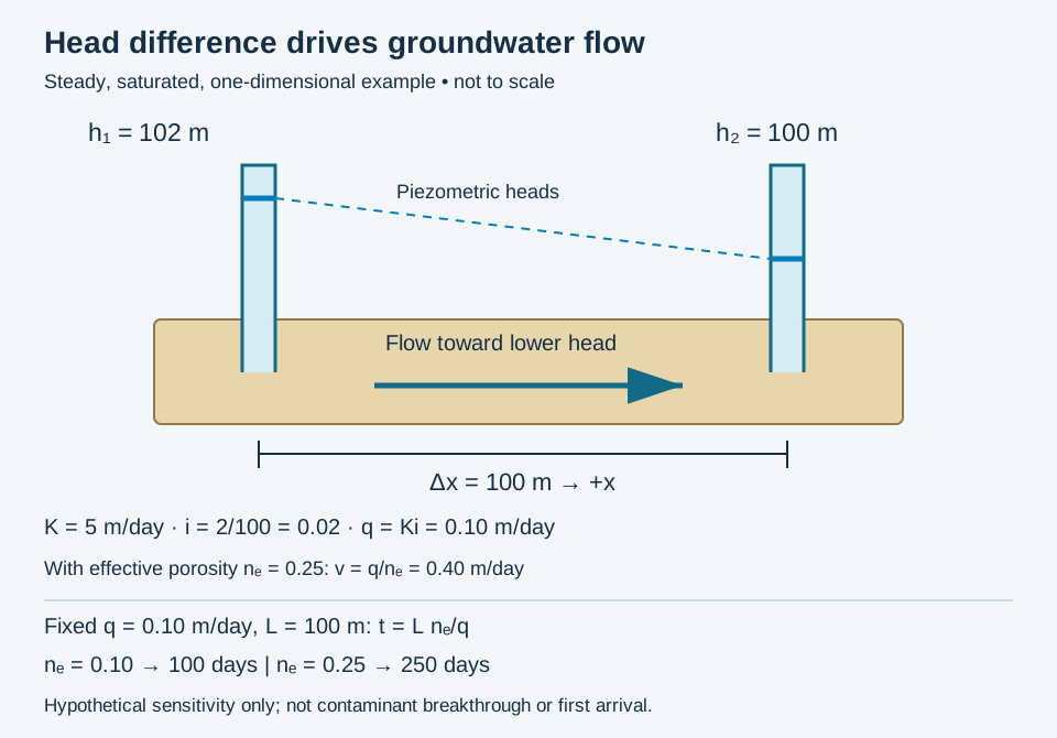
1. Head-loss magnitude: 102 − 100 = 2 m.
2. Gradient magnitude: i = 2 m / 100 m = 0.02.
3. Darcy flux: q = Ki = 5 × 0.02 = 0.10 m/day, toward lower head. With x increasing rightward, dh/dx = −0.02 and q = −K dh/dx.
4. Average advective speed: v = q/ne = 0.10 / 0.25 = 0.40 m/day.
5. Illustrative travel time: 100 / 0.40 = 250 days if those properties remain uniform along the whole path.

The travel time is a bulk advection estimate. It is not a prediction of contaminant arrival, which can differ because of dispersion, sorption, reactions or preferential pathways. Darcy flux uses the entire cross-section; average pore-water speed uses the effective flow fraction.

Do not substitute drainage storage for flow porosity

Specific yield concerns gravity-drainable water per bulk volume. Specific retention concerns water left after drainage. Neither is automatically the effective flow porosity needed for this velocity estimate. Drainage time matters, especially in fine sediment.

Review before using field measurements

• Check datum, units, screen intervals and whether levels have stabilized.
• Distinguish isolated perched zones from a hydraulically connected interval.
• Review density differences before interpreting fresh-water and saline-water heads together.
• Do not extrapolate this uniform example through a fractured or layered reservoir without evaluating heterogeneity and anisotropy.

Sources and scope

Compiled by GeoNavigate from the references below; original hypothetical calculation. No independent expert-review claim is made.

• The Groundwater Project: Darcy’s law, flux and velocity
• Freeze and Cherry: physical properties and principles
• USGS: estimating specific yield

For geological supervision and interpretation workflows, see Chaser’s wellsite geology services or contact the team.

Flow-porosity sensitivity: the same flux can give different travel times

Keep the hypothetical segment above unchanged: length L = 100 m, conductivity K = 5 m/day and gradient magnitude i = 0.02. Thus Darcy flux q = 0.10 m/day. Change only the assumed effective flow porosity, nₑ. This isolates one input; it does not describe two measured aquifers.

• At nₑ = 0.10, v = 0.10/0.10 = 1.0 m/day and t = 100/1.0 = 100 days.
• At nₑ = 0.25, v = 0.10/0.25 = 0.40 m/day and t = 100/0.40 = 250 days.

Combining v = q/nₑ and t = L/v gives t = L nₑ/q. In this fixed-flux calculation, increasing nₑ by a factor of 2.5 increases estimated travel time by the same factor. A lower connected flow volume carries the same discharge at a greater average speed. In real materials, conductivity and flow porosity may change together; do not treat this isolated sensitivity as a universal rock trend.

Keep the calculation traceable

Record the source of the porosity estimate, the flow-path length and the basis for assuming steady uniform flow. Do not insert a total-porosity or drainage-storage number without checking whether it represents the moving-water fraction. These two stipulated inputs are not a confidence interval. The calculated times describe bulk advection, not the earliest detectable solute or its peak concentration. Dispersion, preferential pathways and chemical interactions need separate assessment.

The shared full-size schematic includes both sensitivity results. Compare average linear velocity, Darcy flux and porosity conventions. Concept source: The Groundwater Project, Darcy’s law and average linear velocity, checked 29 October 2026. Original hypothetical calculations, not field data or an expert-reviewed forecast. For geological support, see Chaser services.

Gaining or losing: a streambed head-reversal example

A gaining reach receives groundwater; a losing reach sends water into the subsurface. These labels can change along a channel or through time. They do not classify the entire river permanently. USGS Circular 1139 distinguishes connected losing reaches from those separated from groundwater by unsaturated sediment.

Hold the bed properties fixed

Consider two invented steady end states of one saturated streambed patch. Set bed-top elevation z = 99.0 m, bed-bottom elevation z = 98.5 m and stream water-surface elevation 100.0 m, all on one datum with z positive upward. Neglect velocity head and take stream head at the bed top as 100.0 m. Let bed thickness b = 0.50 m, vertical hydraulic conductivity Kz = 0.010 m/day and horizontal bed area A = 100 m². Assume constant-density water, uniform bed properties, vertical flow and no additional head loss outside the modelled bed.

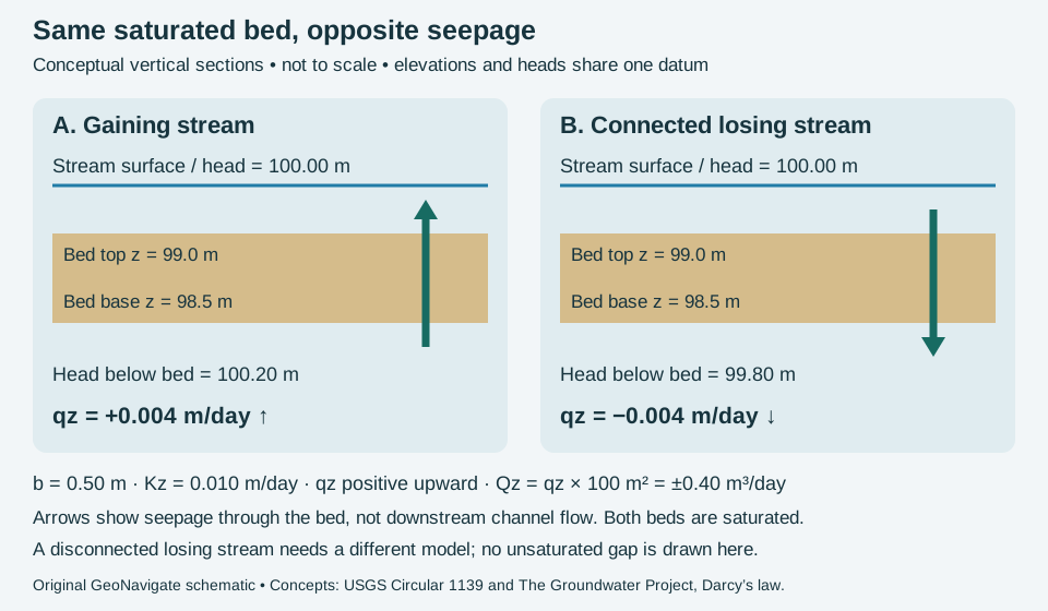
The signed upward flux is qz = −Kz (h_top − h_bottom)/b. With h_bottom = 100.20 m, the gradient is −0.40 and qz = +0.004 m/day: groundwater enters the stream. With h_bottom = 99.80 m, the gradient is +0.40 and qz = −0.004 m/day: the stream loses water downward. Multiplying by area gives +0.40 or −0.40 m³/day. These are exchanges across the modelled bed patch, not total river discharges or pore-water velocities.

Test the limits before scaling up

Both bottom pressure heads remain positive: h − z is 1.70 m in the gaining case and 1.30 m in the losing case. Thus a lower groundwater head than stream stage does not by itself imply an unsaturated gap. For a disconnected losing stream, the saturated-column assumptions fail; do not extend this linear formula by inserting an arbitrarily deeper regional water table.

A real reach requires spatially distributed evidence, bed-property estimates and synchronized stage and piezometer observations. Runoff, tributaries, withdrawals and storage changes can affect a measured downstream discharge difference. The original calculation here isolates bed seepage; it is not a water-budget closure or an assessment of any actual drilling location. Compare oilfield terminology and Chaser Geological services.

Concept sources checked 30 October 2026: USGS Circular 1139, stream–groundwater interactions; The Groundwater Project, groundwater connection with streams; Darcy’s law and specific discharge. No publication artwork or private field data is reproduced.

Vertical gradient: higher head can occur deeper

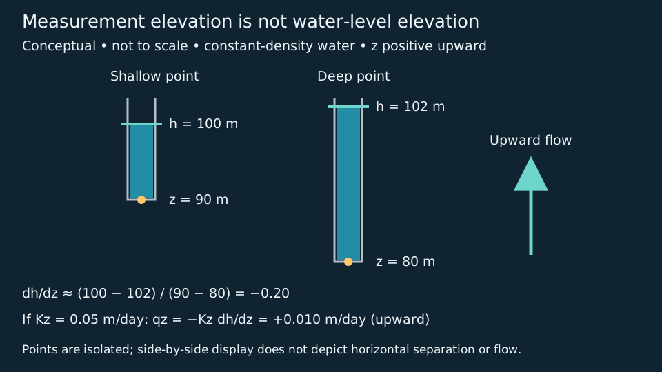
Compare piezometer measurement elevations with their water-level elevations. These are different quantities. Adopt elevation z positive upward and one common datum.

Calculate with a stated coordinate convention

Stipulate a shallow point at z = 90 m with h = 100 m and a deep point at z = 80 m with h = 102 m. The finite-difference estimate is (100 − 102)/(90 − 80) = −0.20. For uniform vertical conductivity Kz = 0.05 m/day and one-dimensional steady flow, qz = −0.05 × (−0.20) = +0.010 m/day. Positive flux points upward. This is a Darcy flux, not pore-water speed.

The corresponding pressure heads h − z are 10 m and 22 m. Neither pressure head alone nor the greater depth alone identifies flow direction. If the deep head instead equalled 100 m, the vertical head gradient would be zero despite unequal pressures.

What the idealized pair leaves unresolved

Separate isolated intervals are essential to this interpretation. A long screen can mix hydraulic responses; assigning its reading to a midpoint does not restore a missing depth profile. Report screen intervals, seals, datum, observation times and stabilization. The two-point result is an average gradient, not proof of uniform properties between points. Density contrasts, lateral gradients and anisotropy need additional analysis. This groundwater calculation does not supply a drilling mud-weight window or an influx forecast.

Concept references checked 29 October 2026: Cohen and Cherry, Darcian Head Profiles and EPA, Vertical Gradient Calculator: screen-length assumptions. Calculations and artwork are original educational material, not field measurements or an external expert review. Continue to oilfield terminology, datum reconciliation or Chaser services.

Depth to water is not hydraulic head: reconcile the datum first

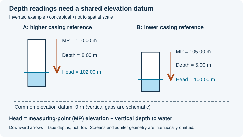
A tape reading is a distance below a marked measuring point. Head is an elevation referenced to a datum. For the nonflowing wells in this invented example, subtract vertical depth to water from measuring-point elevation. Assume stabilized observations taken at the same time, equal water density and screens connected to the same hydraulic unit.

Work the subtraction before interpreting flow

• A: measuring-point elevation 110.00 m; depth to water 8.00 m; head = 102.00 m.
• B: measuring-point elevation 105.00 m; depth to water 5.00 m; head = 100.00 m.
• For a hypothetical one-dimensional horizontal segment of length 100 m from A to B, signed gradient = (100 − 102)/100 = −0.020. With positive scalar conductivity, the Darcy-flow component is toward B.

The deeper tape reading at A does not mean lower head. Comparing only the negative depths would give (−5 − (−8))/100 = +0.030, reversing the sign and changing the magnitude. This is a datum error, not evidence for a reversed groundwater gradient.

What two measurements cannot tell you

The one-dimensional condition is an explicit teaching assumption. Two wells alone do not establish the full horizontal head-gradient vector; an anisotropic conductivity tensor can also rotate flow relative to the gradient. Different screen intervals may sample separate hydraulic units. Do not join their water levels into a water-table surface without that geological evidence.

Keep the marked casing reference, surveyed elevation, vertical datum, tape corrections, observation time and screen interval with each reading. Depth below ground is not depth below casing. Do not use drilled measured depth as a vertical water-level distance in an inclined hole. Flowing wells and pressure transducers require their appropriate pressure-reference and instrument corrections.

As an independent uncertainty exercise, suppose each calculated head has a worst-case bound of ±0.10 m. The A-minus-B difference is then 2.00 ±0.20 m and the 100 m directional gradient magnitude ranges from 0.018 to 0.022, ignoring distance uncertainty. Those bounds are not a statistical confidence interval. If the nominal head difference were only 0.10 m with the same bounds, its sign would be unresolved.

References and related learning

Concept references checked 28 October 2026: Groundwater Project: Hydraulic Head and Measuring and Recording Water Levels. Calculations and schematic are original teaching material, not published field results or an expert-reviewed site assessment. Compare hydraulic head, hydraulic gradient and the Oilfield Glossary. For support, see Chaser services or contact GeoNavigate.

Worked transport example: water speed is not solute speed

Sorption includes attachment to a surface (adsorption) and uptake into a phase (absorption). Reversible exchange can delay a substance while preserving its total mass. That differs from degradation, which transforms the substance. This distinction matters when interpreting groundwater samples near an operating site or comparing a tracer test with a flow model.

Define the coefficient before calculating

The sorption distribution coefficient Kd = Cs/Cw compares sorbed concentration Cs in mg/kg of dry solid with dissolved concentration Cw in mg/L of water. The resulting unit is L/kg, not a dimensionless mass fraction. A constant coefficient assumes a linear equilibrium relation over the chosen concentration range. It is distinct from mineral–melt partitioning used in igneous geochemistry.

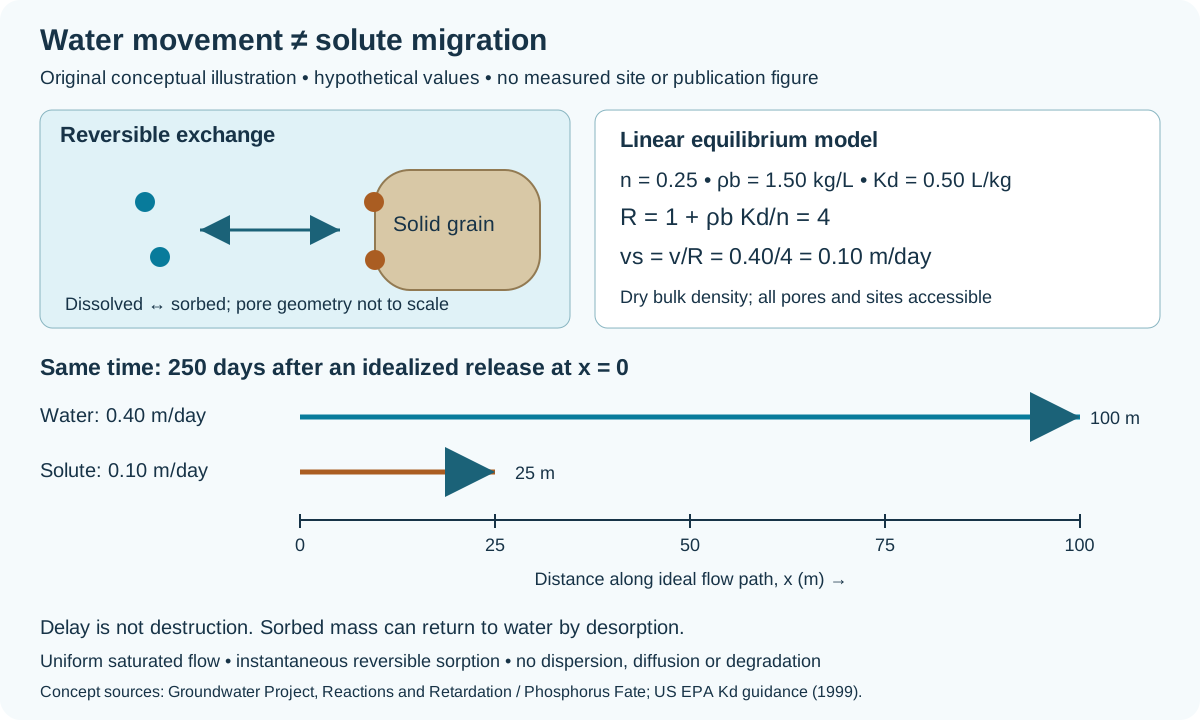
Use the preceding example's pore-water speed v = 0.40 m/day. For this additional hypothetical case, assume saturated homogeneous material, total and effective porosity both n = 0.25, dry bulk density ρb = 1.50 kg/L of bulk material, and Kd = 0.50 L/kg. All pores and sorption sites are accessible. Exchange is instantaneous, reversible and linear; chemistry and flow stay constant. Ignore dispersion, diffusion and degradation. These are teaching assumptions, not a measured contaminant or site forecast.

1. Retardation: R = 1 + ρb Kd/n = 1 + (1.50 × 0.50)/0.25 = 4. The density must be dry solid mass per bulk volume, not grain density.
2. Solute migration speed: vs = v/R = 0.40/4 = 0.10 m/day.
3. Travel over 100 m: water takes 100/0.40 = 250 days; the idealized solute takes 100/0.10 = 1,000 days.
4. Same elapsed time: after 250 days, the ideal water displacement is 100 m and the solute displacement is 25 m. These are characteristic transport positions, not individual molecular paths or a first-detection threshold.

A mass-balance check, not a removal claim

At an invented equilibrium Cw = 2 mg/L, Cs = 0.50 × 2 = 1 mg/kg. One litre of bulk material contains 0.25 L water and 1.50 kg dry solids. Dissolved mass is 0.25 × 2 = 0.50 mg; sorbed mass is 1.50 × 1 = 1.50 mg; total mass is 2.00 mg. The solid holds 75% of that inventory in this example, but nothing has been destroyed. Desorption can return mass to the water when conditions change.

When the simple model stops being adequate

Real breakthrough curves can spread and tail. A single retardation factor does not encode preferential flow, inaccessible pore water, slow exchange, nonlinear sorption or changing pH and competing ions. EPA emphasizes using coefficients appropriate to the actual solids and water chemistry. Review concentration range, equilibration time and porosity convention before applying a batch result to a geological interval. This example cannot establish cleanup time, acceptable exposure or permanent immobilization.

Original explanation and arithmetic checked 26 October 2026; no expert review claimed. Compare the pore-volume accounting example and Oilfield Glossary, or visit Chaser Geological services and contact GeoNavigate.

Worked example: the head-drop direction is not always the flow direction

A contour map describes hydraulic head. Turning it into a flow-direction estimate also requires a model of the medium. Isotropy concerns direction at one location; homogeneity concerns changes between locations. Specify the property and scale before using either description. Horizontal isotropy does not establish equal vertical conductivity.

Choose principal axes and explicit signs

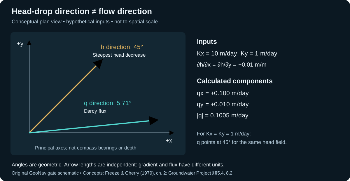
Use an invented homogeneous, saturated medium in two-dimensional plan view, with constant-density water and Darcy flow. Local principal axis x points right and y points up on the page; neither is a compass bearing or depth. Take Kx = 10 m/day and Ky = 1 m/day. Let h = 100 − 0.01x − 0.01y metres, with x and y in metres relative to an arbitrary origin. Thus both partial head derivatives are −0.01 m/m. The direction of steepest head decrease, −∇h, has components (+0.01, +0.01), at 45° counterclockwise from +x.

In these principal axes the conductivity tensor has no off-diagonal terms. Apply qx = −Kx ∂h/∂x and qy = −Ky ∂h/∂y: qx = +0.100 m/day; qy = +0.010 m/day. The flux direction is atan2(0.010, 0.100) = 5.71° from +x. Its magnitude is √(0.100² + 0.010²) = 0.1005 m/day. These are specific-discharge components, not individual pore-water speeds.

Check the result rather than just the arrow

At x = 10 m, y = 0 m, head is 99.90 m; at x = 0 m, y = 10 m it is also 99.90 m. Equal coordinate head drops therefore coexist with unequal flux components. The calculated q · ∇h is −0.0011 m/day: head decreases along the flux direction, even though that direction is not the steepest decrease. This is a local consistency check, not a travel-time prediction.

For a comparison with Kx = Ky = 1 m/day, the same head field gives q = (0.010, 0.010) m/day, at 45°. Conversely, an anisotropic medium can still have parallel flux and negative-gradient directions when the gradient lies on a principal axis. A single aligned observation is not proof of isotropy.

Before applying this to an aquifer

Check whether mapped heads represent the same connected interval and datum. Record conductivity-test directions and their scale. If principal axes are rotated relative to the map, transform the tensor rather than substituting its principal values directly into the map-coordinate equations. This two-dimensional exercise does not resolve vertical flow, fractures below the continuum scale, density-driven flow or a contaminant travel path. Compare the layered-conductivity example for a different source of bulk anisotropy.

References and provenance

Checked 27 October 2026: Groundwater Project §5.4 (direction versus location); Freeze and Cherry, Groundwater, chapter 2 (generalized Darcy law and tensor); Groundwater Project §8.2 (flow-direction interpretation). Original explanation, arithmetic and artwork; no measured result or expert review claimed. Continue in the Oilfield Glossary, explore Chaser Geological services or contact GeoNavigate.

Solute spreading: velocity, dispersivity and units

A groundwater velocity estimate describes average movement. It does not say that every dissolved molecule follows the same route or arrives together. Mechanical dispersion represents spreading associated with differing flow velocities and paths. Molecular diffusion supplies another contribution, driven by concentration differences. Here, “hydrodynamic dispersion” means their combined effect; terminology varies between sources.

Worked example: calculate coefficients, not a plume boundary

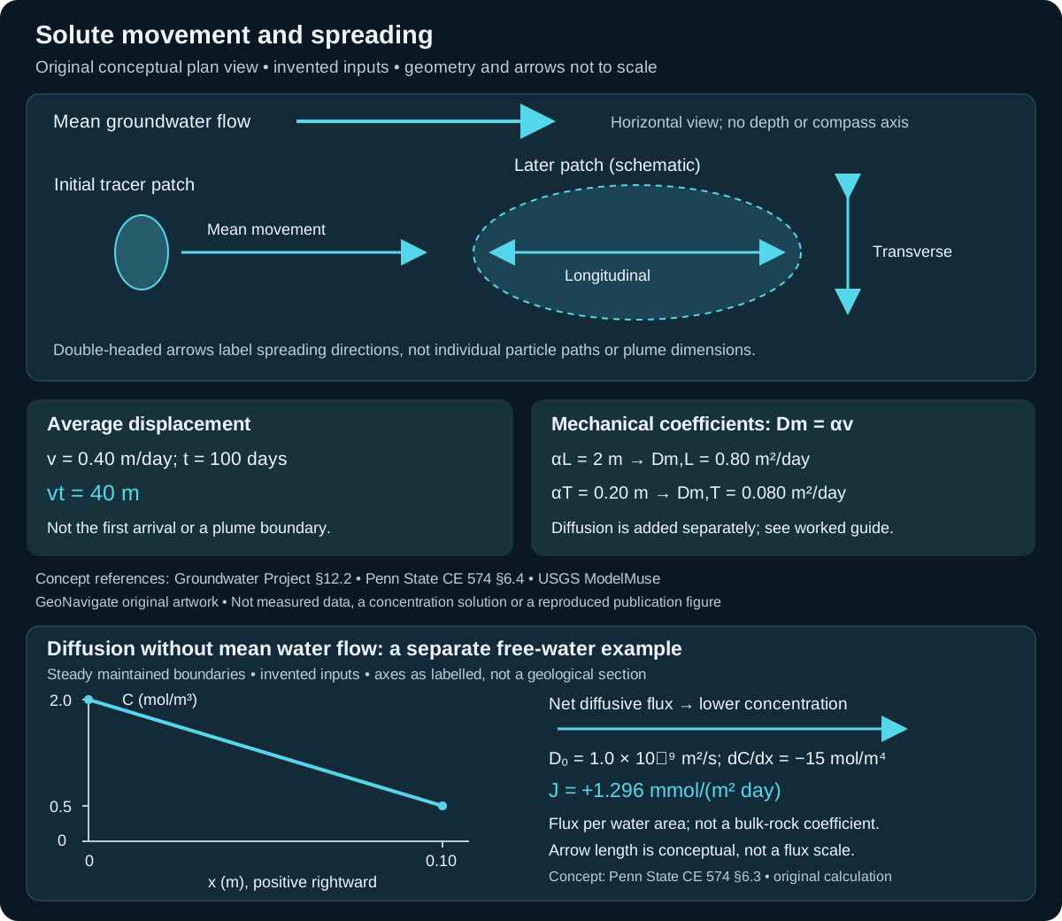
Consider a separate hypothetical, saturated medium with steady uniform mean flow to the right. Use average pore-water speed v = 0.40 m/day, longitudinal dispersivity αL = 2 m and horizontal transverse dispersivity αT = 0.20 m. The latter two are invented model inputs, not values inferred from the preceding Darcy example or recommended for a field site. Ignore sorption, reaction, decay and density-driven flow for this exercise.

1. Average advection over 100 days: vt = 0.40 × 100 = 40 m. This is an average displacement, not a first-arrival distance.
2. Longitudinal mechanical coefficient: Dm,L = αL v = 2 × 0.40 = 0.80 m²/day.
3. Transverse mechanical coefficient: Dm,T = αT v = 0.20 × 0.40 = 0.080 m²/day. The coefficient ratio is ten; that does not make a plume ten times as long as it is wide.

The unit check is m × m/day = m²/day. A dispersivity is a length; a coefficient is a length squared per time. Neither is a plume width. To calculate concentrations, specify the source history, initial and boundary conditions, flow field and transport equation.

For a separate illustration of addition, assume an effective molecular diffusion coefficient De = 0.00010 m²/day, equal in both directions. Then DL = 0.80010 and DT = 0.08010 m²/day. These are total coefficients under the stated model. Holding De fixed while reducing v reduces the mechanical contribution, so ignoring diffusion cannot be justified from a high-speed example alone.

Interpretation checks before using a model

• Use pore-water speed, not Darcy flux, in the stated coefficient formula.
• Document calibration distance and geological heterogeneity. A column-derived dispersivity may not describe a field-scale plume.
• Distinguish longitudinal and transverse directions relative to flow. This plan view shows only horizontal spreading; vertical transport needs its own treatment.
• Check solver definitions and numerical spreading. USGS ModelMuse documents separate direction-dependent inputs and warns that model horizontal and vertical axes do not automatically rotate with dipping beds.
• Keep physical spreading separate from sorption retardation, transformations and source-duration effects. A delayed or broadened signal alone does not identify one mechanism.

References and scope

• The Groundwater Project, Basic Hydrogeology §12.2 — advection and spreading mechanisms.
• Li Li, Penn State CE 574 §6.4, Dispersion — coefficient relation, units and diffusion contribution.
• USGS ModelMuse, GWT Dispersion Package — direction conventions and model limitations.
• Freeze and Cherry (1979), Groundwater §9.2 — transport assumptions and concentration histories.

Original GeoNavigate explanation and artwork; sources checked 27 October 2026. No external expert review claimed. See the Oilfield Glossary entry, Geology Guides, Chaser Geological services or contact Chaser Geological.

Molecular diffusion: a flux even when mean water flow is zero

Molecular diffusion and mechanical dispersion describe different processes. In the simple one-dimensional Fickian model, J = −D₀ dC/dx. Here J is dissolved molar flux per unit water cross-sectional area, C is concentration per water volume, and D₀ is the free-water diffusion coefficient. A concentration gradient can drive net diffusion without an advective water flux.

Worked sign and unit check

Consider a separate, hypothetical water-filled chamber at constant temperature, with no porous solid and no mean water flow. Let x increase rightward. Maintain C = 2.0 mol/m³ at x = 0 and C = 0.5 mol/m³ at x = 0.10 m. Stipulate a constant D₀ = 1.0 × 10⁻⁹ m²/s for a dilute, nonreacting neutral solute. Assume a steady linear concentration profile; these are teaching inputs, not a measured chemical system.

1. Gradient: (0.5 − 2.0)/0.10 = −15 mol/m⁴.
2. Flux: J = −(1.0 × 10⁻⁹)(−15) = +1.5 × 10⁻⁸ mol/(m² s). The positive sign means rightward, from higher to lower concentration.
3. Daily conversion: J × 86,400 = 0.001296 mol/(m² day), or 1.296 mmol/(m² day).

For a water cross-section of 0.020 m², the transfer rate is 0.02592 mmol/day. Multiplying by area gives amount per time; dividing by concentration is not needed to obtain this rate. The shared full-size schematic plots the two boundary values and the assumed linear profile.

Reverse the gradient, not the diffusion coefficient

Swapping the boundary concentrations reverses J while D₀ remains positive. Equal boundary concentrations give zero net Fickian flux in this uniform steady example; individual molecules still move. In a closed finite chamber, concentrations evolve and a constant-flux extrapolation would fail. The fixed boundaries above require maintained reservoirs.

Transfer the concept to rock cautiously

Porous rock adds restricted pathways and a choice of flux-area convention. Check a model’s definition of effective diffusion and its placement of porosity before inserting a free-water coefficient. Do not multiply by porosity twice. This chamber example contains no sorption, electrical coupling, density circulation or reaction; it supplies no aquifer breakthrough time. Compare oilfield usage and hydraulic diffusivity, which concerns pressure or head response rather than molecular mixing.

Concept reference: Li Li, Penn State CE 574 §6.3, Diffusion, read 30 October 2026. The values, arithmetic and schematic are original GeoNavigate educational material; no source figure or private data is reproduced. For geological interpretation support, see Chaser services or contact Chaser Geological.

Worked example: a confining layer can still leak

An aquitard limits groundwater transmission without necessarily stopping it. The Bureau of Reclamation field manual distinguishes this hydraulic role from a productive aquifer. Here we test a simple vertical-flow model; all numbers and geometry are invented.

Calculate the quantity you actually need

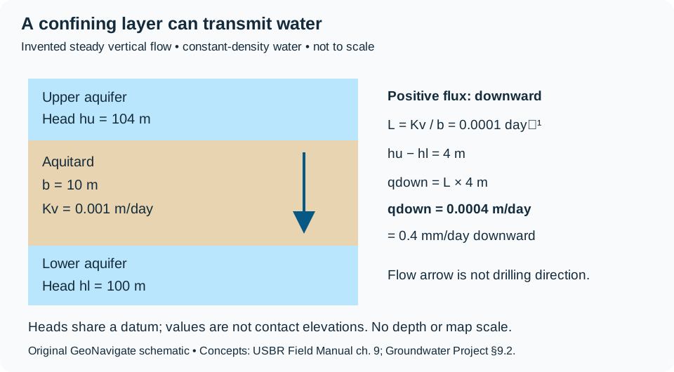
Assume saturated, homogeneous material, constant-density water, steady one-dimensional vertical flow, fixed boundary heads and no bypass. Let vertical hydraulic conductivity Kv = 0.001 m/day, aquitard thickness b = 10 m, upper-boundary head hu = 104 m and lower-boundary head hl = 100 m. Choose positive flux downward.

1. Vertical leakance: L = Kv/b = 0.001/10 = 0.0001 day⁻¹.
2. Head difference: hu − hl = 4 m. Thus qdown = L(hu − hl) = 0.0004 m/day, or 0.4 mm/day.
3. Across a hypothetical uniform area of 1,000 m², conductance A × L = 0.1 m²/day and total flow Q = A × qdown = 0.4 m³/day.

The Groundwater Project defines vertical leakance as conductivity divided by thickness. Keep its inverse-time units separate from Darcy flux (length/time) and flow rate (volume/time). The area is a stipulated horizontal footprint, not the cross-section of a well. This calculation estimates leakage through the entire assumed footprint, not a borehole influx rate.

Reverse the head difference, then change the layer

In a separate steady state with hu = 98 m and hl = 100 m, qdown = −0.0002 m/day: flow is upward. Vertical position alone does not set direction; compare total heads. Returning to the original 4 m difference but doubling b to 20 m halves leakance and flux if Kv stays unchanged. Neither change gives a travel time or the time needed to reach that new steady state.

What would make the model inadequate?

A fracture crossing the layer, an erosional window or contrasting sublayers can defeat a uniform-medium approximation. A USGS-listed study of the St. Lawrence Formation describes how fracture connectivity and local geological setting influence aquitard integrity. That regional result supports examining pathways; it supplies no calibrated conductivity for this invented example or an Alberta well.

For field interpretation, check isolated measurement intervals, equilibration, head datum, density and the spatial support of the conductivity estimate. A gamma-ray-rich interval alone supplies none of these hydraulic boundary conditions. Pressure changes can involve storage as well as leakage. Do not use this exercise to specify mud weight, a fracture limit or loss-control treatment. Distinguish the geological interpretation from a site-specific drilling assessment.

Original GeoNavigate explanation and schematic, sources checked 28 October 2026. No publication figure or measured result reproduced; no external expert review claimed. Compare the Oilfield Glossary entry and Chaser wellsite geology services.