
GEONAVIGATE / RESOURCES / GEOLOGICAL TIME
Radiometric dating and cooling histories
Work through half-life and cooling-rate examples, distinguish mineral ages from depositional ages, and understand closure-temperature assumptions.
First ask which event the age records
A mineral age is evidence about a particular geological event. Crystallization, cooling and later alteration can leave different isotopic records. Before comparing an age with a formation top, identify the dated mineral, the isotope system, the sample context and the laboratory's interpretation. A number without those details cannot safely be treated as a depositional age.
Work through a deliberately simple decay system
For this invented example, one parent atom becomes one stable daughter atom, there is no initial daughter, and no relevant atoms enter or leave the sample. This is a teaching model, not a specific real isotope pair or a laboratory calibration. Let P be parent atoms remaining and D* be daughter atoms produced by decay. The asterisk excludes any initial daughter.
After one half-life, half the parent remains. After two, one quarter remains. After three, one eighth remains. The elapsed time is t = T½ × log₂(1 + D*/P), where T½ is the half-life. This expression applies to our single-step, closed system.
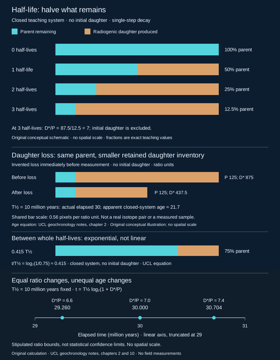
Calculate an age, then challenge the assumptions
Suppose the hypothetical half-life is 10 million years and corrected atom counts give P = 125 and D* = 875. Then D*/P = 7, log₂(8) = 3 and t = 30 million years. These small counts are illustrative ratios, not actual laboratory sample sizes or precision estimates.
Now suppose the measured total daughter count is 1,000, of which 125 atoms were present initially. Subtracting that initial component still leaves D* = 875. Incorrectly treating all 1,000 daughter atoms as radiogenic gives 10 × log₂(9) ≈ 31.7 million years. The extra apparent age comes from a mistaken starting condition, not extra elapsed time.
A closed system is an assumption to test
A closed isotopic system retains the relevant parent and daughter atoms. Daughter loss, parent gain, inherited grains and partial resetting can complicate an age. Different minerals and isotope systems respond differently to heating and fluids. Laboratory methods may estimate initial components from isotope ratios or use multiple decay systems; our simple calculation does not replace those methods. Report uncertainties and geological qualifications with the age.
Bracket a sedimentary interval with suitable ash beds
Imagine an undisturbed sedimentary sequence with a primary ash bed below the interval dated at 105 Ma and another above dated at 101 Ma. If the selected crystals date those eruptions and the ash was deposited promptly without reworking, the intervening sediment was deposited after 105 Ma and before 101 Ma: its numerical age lies between 101 and 105 Ma. Older ages have larger Ma numbers. Dating uncertainty broadens the bracket; an unconformity may represent missing time.
A 250 Ma detrital zircon in the same sediment instead records part of the source history. It does not make the sediment 250 Ma old. Even the youngest grain or grain population requires checks for analytical reliability, inheritance, disturbance and sampling before it is used as a maximum depositional-age constraint. Cross-check with radiometric dating, stratigraphic order and fossil preservation and reworking.
Use ages in wellsite correlation without overstating them
- Record the sample depth, mineral, dated material and whether it is primary or reworked.
- Separate the analytical age from the interpreted event and its uncertainty.
- Check whether the age constrains a source rock, eruption, cooling history or sedimentary interval.
- Retain conflicting fossil, log and stratigraphic evidence for review rather than forcing a numerical match.
Sources and scope
- USGS: Radiogenic Isotopes and the Eastern Mineral Resources Program — isotope tracers and closed-system assumptions.
- Steven Earle / BCcampus: Isotopic Dating Methods — mineral dating and sedimentary age constraints.
- University of Saskatchewan Physical Geology: Isotopic Dating Methods — selecting minerals and bracketing sedimentary rocks.
Original explanation, invented examples and vector artwork prepared 25 October 2026. No expert review or measured sample is claimed. Explore the Geology Dictionary, Oilfield Glossary, Chaser wellsite services or contact GeoNavigate.
Pooling isotope amounts is not averaging ages
Suppose two components follow the same invented single-step parent–daughter system, each remained closed before pooling, and neither contained initial daughter. Use a hypothetical half-life of 10 million years. P and D* below are proportional atom amounts on one common scale, not laboratory counts or mass fractions.
| Component | P | D* | D*/P | Calculated age |
|---|---|---|---|---|
| A | 100 | 100 | 1 | 10 million years |
| B | 100 | 700 | 7 | 30 million years |
| Pooled amounts | 200 | 800 | 4 | 23.22 million years (apparent) |
Using the UCL age equation, t = T½ log₂(1 + D*/P), A gives 10 log₂(2) = 10 and B gives 10 log₂(8) = 30 million years. Pool the amounts first: (100 + 700)/(100 + 100) = 4. Inserting that ratio gives 10 log₂(5) ≈ 23.2193 million years. The arithmetic mean of the two ages is 20 million years. These are different operations.
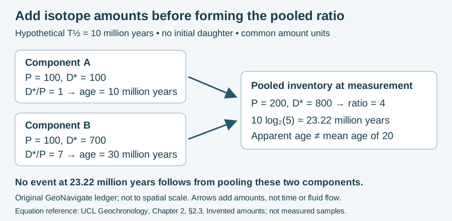
Keep the calculation separate from its geological meaning
Equal present parent amounts make the pooled ratio the simple mean of ratios 1 and 7 in this example. In general, ratios must be weighted by their parent amounts: r pooled = (Pₐrₐ + Pᵦrᵦ)/(Pₐ + Pᵦ). Equal sample masses do not establish equal parent inventories. The logarithmic age transformation means that even an appropriately pooled ratio does not normally yield an arithmetic mean age.
No crystallization, cooling or mixing event at 23.22 million years was stipulated. The pooled number therefore does not establish one. Component selection, inherited domains, initial daughter and isotope-system behaviour require their own evidence. Do not treat this exercise as a method for combining laboratory ages or their uncertainties. Compare radiometric dating, parent isotope and the oilfield dating entry.
Equation source checked 31 October 2026: UCL geochronology notes, Chapter 2, §2.3, linked above. The pooling scenario, values and schematic are original teaching material; no private sample data or external expert review is claimed. Contact Chaser Geological.
Worked example: a fraction of a half-life
For the same closed, single-step teaching system with no initial daughter, let 75% of the original parent remain. The elapsed fraction is t/T½ = log₂(1/0.75) ≈ 0.415. With the hypothetical 10-million-year half-life above, this is about 4.15 million years. The new bottom bar uses 420 of 560 pixels for parent and 140 for radiogenic daughter.
A straight line from 100% parent at time zero to 50% at one half-life would put 75% at 0.5 half-lives, or 5 million years. That interpolation is inappropriate for exponential decay. Conversely, at 0.5 half-lives, the remaining fraction is 2^(−0.5) ≈ 70.71%, not 75%.
The initial parent inventory is stipulated here, not normally known from a rock measurement. Real dating requires the isotope system, initial-component treatment, retention history and uncertainty. Equation reference: UCL geochronology notes, section 2.3. Original illustrative calculation; no measured sample or external expert review claimed.
Worked example: daughter loss is not a younger formation event
Continue the invented single-step system above: half-life 10 million years, no initial daughter, P = 125 and radiogenic D* = 875 in proportional atom-count units. Its closed-system age is 30 million years. Now impose a loss of half the accumulated daughter immediately before measurement, retaining all parent. This timing is deliberate: there is no subsequent ingrowth to calculate. The retained D* is 437.5 and D*/P is 3.5.
Blindly applying the closed-system expression gives t = 10 × log₂(1 + 437.5/125) ≈ 21.7 million years. That is an apparent age under an invalid closure assumption, not the known 30-million-year elapsed time. Fractional counts represent normalized amounts, not half an individual atom. The diagram uses the same absolute ratio-unit scale for both cases; the shorter retained total must not be renormalized to look like unchanged inventory.
The arithmetic can be generalized for this particular loss-at-measurement model: if f is the retained fraction of radiogenic daughter, t apparent = T½ × log₂[1 + f(2^(t true/T½) − 1)]. For 0 < f < 1 and unchanged parent, the apparent value is younger. Earlier loss followed by ingrowth, parent exchange, initial daughter and multiple episodes require different models. A single measured ratio cannot identify f or recover a unique true age.
For stratigraphic work, do not move a formation top simply to match the younger number. Check mineral domains, alteration, analytical uncertainties, concordance where applicable and independent stratigraphic evidence. A disturbed grain may still contain useful history, but that interpretation requires the relevant laboratory method. Compare closed isotopic system, radiogenic isotope and the cooling-history discussion on this page.
Original illustrative calculation, 29 October 2026; no measured sample or expert review claimed. Formula reference: UCL geochronology notes, age equation. Interpretation context: Fox and Carter (2020), Heated topics in thermochronology and paths towards resolution (repository abstract). The simple instantaneous-loss scenario is our teaching construction, not a fit to that publication.
Cooling histories: what does the date mean?
Thermochronology uses temperature-sensitive records to investigate thermal evolution. For example, helium produced by radioactive decay may escape while a mineral is hot and become increasingly retained as it cools. This behaviour can help investigate basin reheating, mountain belts and fault histories. Radioactive decay continues during heating and cooling; retention is what changes.
Closure temperature is an effective model concept. It depends on the analytical system, kinetic properties, diffusion domain and cooling history. Do not treat a table value as an exact switch shared by every grain. A simple cooling-age interpretation assumes an appropriate cooling history; reheating, partial loss or mineral alteration can require a more detailed model.
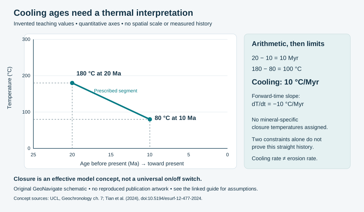
Worked example: a rate with explicit assumptions
Prescribe a hypothetical straight cooling segment between 180 °C at 20 Ma and 80 °C at 10 Ma. The elapsed duration is 20 − 10 = 10 Myr; the temperature decrease is 180 − 80 = 100 °C. The average cooling magnitude is therefore 100/10 = 10 °C/Myr. With elapsed time increasing forward, dT/dt is −10 °C/Myr. Ma labels an age before present; Myr measures duration.
For a sensitivity exercise only, keep the ages exact but allow the older temperature to range from 170 to 190 °C and the younger from 70 to 90 °C. The extreme average magnitudes become (170 − 90)/10 = 8 and (190 − 70)/10 = 12 °C/Myr. This 8–12 range is an arithmetic envelope, not a confidence interval. Actual temperature and age uncertainties may be coupled.
What this calculation cannot establish
Two interpreted constraints do not establish a unique intervening thermal path. The drawn straight line is an assumption. Converting a cooling rate into an exhumation rate also requires a thermal model: subsurface temperatures can vary with heat transport, boundary conditions and topography. No depth, erosion rate or petroleum-generation timing follows directly from this diagram.
For a well or basin report, keep sample depth, mineral/system, measured date and uncertainty, kinetic assumptions and the inferred event in separate fields. Compare a cooling interpretation with independent stratigraphy and thermal evidence. A detrital grain can retain a source history; later burial heating can modify it. State unresolved alternatives rather than silently labelling every date “formation age.”
References and scope
- Pieter Vermeesch, UCL: Thermochronology — helium diffusion, closure and fission-track behaviour.
- Tian, Pan, Zhang and Yao (2024), Earth Surface Dynamics — closure kinetics and thermal-model assumptions in exhumation inversion.
- University of Colorado Boulder TRaIL: (U-Th)/He background — retention and geological applications.
Original explanation and arithmetic checked 26 October 2026; no sample data or expert-review claim. See the wellsite glossary context, geology guides, Chaser Geological services or contact GeoNavigate.
Magnetic polarity: separate a rock pattern from its age
A polarity zone describes rock; a polarity chron describes time. Recognizing normal and reversed intervals does not yet identify a unique position on a reference timescale. Use magnetostratigraphy alongside independent fossil or radiometric constraints.
IODP Expedition 396 compared demagnetized core measurements with discrete-sample directions and used biostratigraphic horizons in its age correlation. Core-end reversals were treated cautiously. These are useful examples of evidence checks, not a universal laboratory recipe. Preserve the sample orientation and depth convention, disturbance observations, demagnetization results, proposed tie and chosen timescale edition.
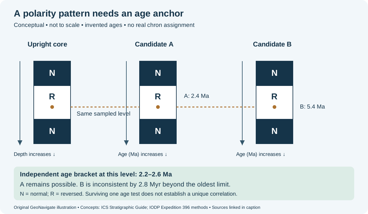
Worked example: test two possible correlations
Imagine an upright, continuously recovered core with an interpreted normal–reversed–normal pattern downward. A provisional correlation places its middle sampled level at either 2.4 Ma (candidate A) or 5.4 Ma (candidate B). These are invented alternatives, not named geomagnetic chrons.
Now suppose independent evidence constrains that same level to 2.2–2.6 Ma. Candidate A falls inside the bracket; candidate B is older than its oldest limit by 5.4 − 2.6 = 2.8 Myr. Under the stated assumptions B is inconsistent. A survives this test, but is not proved unique: another correlation might also satisfy the bracket. Do not give it a probability from this arithmetic.
Locate a boundary without inventing precision
In a separate hypothetical sampling exercise, reliable samples at 12.0 m and 12.5 m core depth have opposite polarity. With continuous undisturbed recovery, a genuine single transition is bracketed within that 0.5 m interval. A pick at 12.25 m is only the midpoint convention, not a measured reversal depth. Additional transitions between samples remain possible. Do not convert this depth bracket into years without an age–depth model.
Challenge the geological interpretation
A later magnetic overprint can record heating or alteration rather than deposition. Keep a descriptive polarity unit distinct from its inferred history. Missing section or disturbed core can also complicate pattern matching. Report unresolved ties and what evidence could discriminate them, rather than assigning a familiar chron name from one normal interval.
Original explanation and invented arithmetic checked 26 October 2026; no expert review claimed. Continue to wellsite terminology, geology guides, Chaser Geological services or contact GeoNavigate.
Detrital zircon: turn an age into a bound
A detrital zircon is a transported grain, not a clock started by sandstone deposition. Distinguish the dated mineral event from the formation of the bed containing it. The maximum depositional age (MDA) is an older limit: in Ma before present, a valid 105 Ma bound means deposition is no older than 105 Ma. It does not mean deposition occurred exactly then.
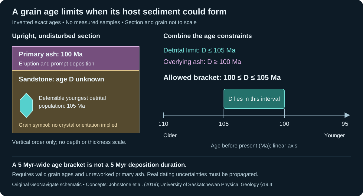
Worked example: combine two different constraints
Let D be the sandstone's depositional age in Ma before present. Prescribe a defensible youngest detrital population age of 105 Ma and an overlying primary ash with an eruption age of 100 Ma. Assume the beds are upright and undisturbed, and that the ash was deposited promptly without reworking. Treat the ages as exact solely to isolate the inequality logic.
- The detrital constraint gives D ≤ 105 Ma: the sediment cannot predate its valid pre-depositional constituent.
- The overlying ash gives D ≥ 100 Ma: the sandstone was already deposited when that ash arrived.
- The intersection is 100 ≤ D ≤ 105 Ma. For example, 103 Ma satisfies both bounds. Neither 108 Ma nor 98 Ma does.
The interval spans 5 Myr, but that is the width of the allowed age bracket, not the duration of sandstone deposition. The bounds alone do not select its midpoint or assign equal probabilities across it. Without the overlying ash or another suitable younger constraint, the 105 Ma MDA alone leaves the younger limit unresolved. Real analytical and geological uncertainties must be propagated; these exact teaching numbers are not a confidence interval.
Check the youngest component before using it
Document how the youngest defensible age was estimated and why the selected grains belong to the sample. Dickinson and Gehrels (2009) compared alternative youngest-age measures against independent biostratigraphy; results depended on the estimator. A single small age is therefore not a universal rule for selecting an MDA. Johnstone and colleagues discuss analytical scatter, contamination and isotope loss, and show why stratigraphic context matters.
At the wellsite, record the sampling interval and whether material is core or cuttings, retain its sample provenance, and keep the laboratory age separate from the interpreted bed age. If the ash is reworked or the succession is fault repeated or overturned, reassess the assumed order before applying this bracket. Compare with chronostratigraphic correlation and fossil evidence rather than forcing an age into a preferred formation assignment.
References and scope
- Johnstone, Schwartz and Holm-Denoma (2019), A Stratigraphic Approach to Inferring Depositional Ages From Detrital Geochronology Data — primary full paper, DOI 10.3389/feart.2019.00057.
- Dickinson and Gehrels (2009), Colorado Plateau Mesozoic test — University of Arizona abstract and metadata, DOI 10.1016/j.epsl.2009.09.013; full paper not reviewed here.
- University of Saskatchewan Physical Geology, §19.4 — mineral ages, sedimentary fragments and relative-age constraints.
Original explanation and arithmetic. Checked 27 October 2026; no expert review claimed. See the separate Oilfield Glossary entry, geology guides, Chaser Geological services or contact GeoNavigate.
Worked example: ratio bounds and asymmetric age bounds
Retain the invented closed, single-step system used above: no initial daughter, one stable daughter per parent decay, and an exactly stipulated half-life T½ of 10 million years. Define r = D*/P using radiogenic daughter only. The elapsed time is t = 10 log₂(1 + r) million years. This model is a calculation exercise, not a calibrated geological clock.
Suppose a sensitivity check brackets r between 6.6 and 7.4 around a nominal value of 7.0. Substitution gives t(6.6) = 29.260 million years, t(7.0) = 30.000 million years and t(7.4) = 30.704 million years. The ratio changes are equally spaced at ±0.4, but the age changes are approximately −0.740 and +0.704 million years. The logarithm is increasing and curved; it does not preserve equal spacing.
The lower panel of the shared decay schematic plots those ages on one linear numerical axis. No depth, map orientation or spatial scale is implied. These are stipulated input limits, not one-sigma, two-sigma or 95% confidence bounds. Assigning a probability requires a measurement model that this example does not supply.
Compare an exact endpoint calculation with local sensitivity
At r = 7, the slope is dt/dr = T½ / [(1 + r) ln 2] ≈ 1.8034 million years per unit ratio. Multiplying by 0.4 gives about 0.7213 million years, a symmetric first-order estimate of the change near that point. The endpoint calculations show its approximation error. Smaller perturbations improve the local approximation; it is not a substitute for a full uncertainty calculation.
Real parent and daughter measurements may be correlated, and half-life and initial-component estimates also have uncertainty. Do not add their percentage uncertainties or assume independence without justification. Report the laboratory's uncertainty convention and treatment of systematic components. Numerical precision also cannot rescue an invalid closure assumption: compare the daughter-loss example.
For geological correlation, keep the measured age and uncertainty separate from the event interpretation. Neither this bracket nor extra decimal places prove that a grain dates sediment deposition. See radiometric dating, half-life and the oilfield entry.
Equation and uncertainty context: Pieter Vermeesch, UCL age equation, section 2.3 and error propagation, chapter 10, checked 30 October 2026. Values, endpoint calculation and illustration are original hypothetical teaching material; no measured sample or expert review is claimed.