Strike, true dip and apparent dip: a worked section example

One plane, different section slopes

A tilted bed can look nearly flat in one cross-section and steep in another without changing orientation. The section heading determines which slope you see. This matters when comparing a geological map, a well trajectory and an interpreted formation top.

Strike is horizontal within the plane. True dip measures its steepest downward inclination from horizontal. Dip direction is the compass bearing of that descent. An oblique vertical section shows apparent dip.

Read the orientation before calculating

Consider a hypothetical planar contact with north–south strike and true dip 30° east. Its dip azimuth is 090°. Under the Canadian right-hand rule, its strike/dip notation is 000°/30°: facing north, east lies to your right. State the convention when exchanging data; the phrase “right-hand rule” is not used identically everywhere. Specify whether bearings use true, grid or magnetic north.

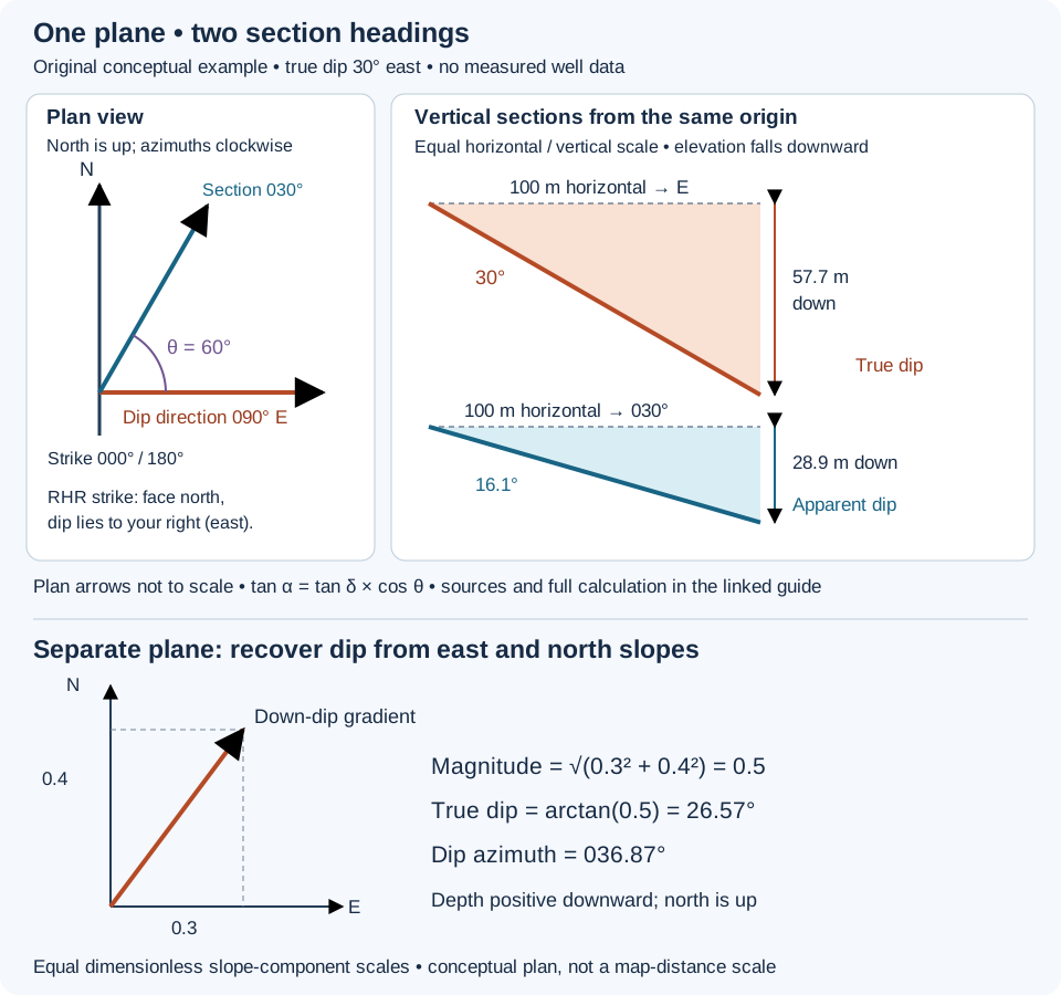
Worked example: a section heading of 030°

Use horizontal distance along the section, not distance measured down a borehole. Let δ be true dip, α the signed slope angle along the section heading, and θ the horizontal angle between that heading and dip azimuth. Take downward change as positive. For a nonvertical plane:

tan α = tan δ × cos θ

This follows by projection. A horizontal step L along the section advances only L cos θ in the down-dip direction. The corresponding downward change is L cos θ tan δ; dividing by L gives the section slope. If instead the acute angle β is measured from strike, the magnitude relation is tan |α| = tan δ × sin β. Do not interchange θ and β.

1. The section heads 030° and the dip azimuth is 090°, so θ = 60°.
2. tan α = tan 30° × cos 60° = 0.288675.
3. α = arctan(0.288675) = 16.1°, rounded.
4. Over 100 m of horizontal section distance, the contact drops 100 × 0.288675 = 28.9 m.
5. Over 100 m due east, it drops 100 × tan 30° = 57.7 m.

These are two different horizontal paths from the same starting point. They do not end at the same map location. With elevation positive upward, the corresponding elevation changes are −28.9 m and −57.7 m. A depth coordinate positive downward reverses those signs.

Checks that catch common interpretation errors

• Along strike: θ = 90° gives zero apparent slope for this nonvertical plane. A flat-looking section does not establish horizontal bedding.
• Down dip: θ = 0° gives the true dip. Reversing the section heading makes the same plane rise instead of fall.
• Vertical exaggeration: if vertical distances are plotted E times larger than horizontal distances, the displayed angle is arctan(E tan α). At E = 2, this example looks 30° steep despite its 16.1° geometric section slope.
• Near strike: recovering true dip requires division by a small projection factor. Small errors in heading or apparent slope can then produce large changes in the inferred true dip.
• Special cases: a horizontal plane has no unique strike or dip azimuth. A vertical plane needs separate treatment; this tangent formula is singular at 90° true dip.

Using the result around a directional well

Apply the projection to a local vertical section with a stated heading. A curved well does not have one heading for its full length. Nor is formation dip the same quantity as well inclination, which is commonly referenced to vertical. Before comparing a projected formation surface with a trajectory, reconcile azimuth reference, depth datum and measured-depth versus vertical-depth coordinates.

The example assumes a single plane. A fold, fault or changing depositional geometry requires separate surfaces or local orientations. An apparent dip estimated from one section cannot, by itself, uniquely determine both true dip and dip direction. Compare independent orientation observations before treating a correlation fit as a measured geological attitude. See the geosteering definition and gamma-ray correlation workflow for related context.

Recover a plane from two perpendicular section slopes

Use a separate hypothetical plane. Let x point east, y north and depth z increase downward, all measured in metres from consistent references. Suppose its depth increases 30 m per 100 m eastward and 40 m per 100 m northward. The plane equation is z = z₀ + 0.3x + 0.4y. These signed slopes correspond to apparent dips arctan(0.3) = 16.70° eastward and arctan(0.4) = 21.80° northward.

The horizontal gradient is (0.3, 0.4). Its magnitude is √(0.3² + 0.4²) = 0.5, so true dip = arctan(0.5) = 26.57°. Its down-dip azimuth, clockwise from north, is arctan(0.3/0.4) = 036.87° in this northeast quadrant. The Canadian right-hand-rule strike is 306.87°. Averaging the two apparent-dip angles would give 19.25°, which is not the true dip.

This reconstruction requires two perpendicular sections of the same planar surface, signed slopes and horizontal distances. For other quadrants use a quadrant-aware atan2(east slope, north slope), normalized to 0–360°. A general nonorthogonal pair needs simultaneous projection equations; do not use the sum-of-squares shortcut. A curved surface, mismatched contacts or uncorrected vertical exaggeration invalidates these inputs. The calculation gives orientation, not the elevation intercept z₀.

Original vector derivation and invented arithmetic. Orientation conventions checked 30 October 2026 against Waldron and Snyder, University of Alberta: Orientation of structures. No source figure or private well data reproduced. Compare dip direction and oilfield apparent dip.

Worked example: remove vertical exaggeration before measuring dip

A section display can stretch depth relative to horizontal distance to make small offsets visible. Vertical exaggeration (VE) describes this scale ratio. It changes the drawn angle, not the contact or the borehole. Check the axis units and scales before using an angle measured on a screen.

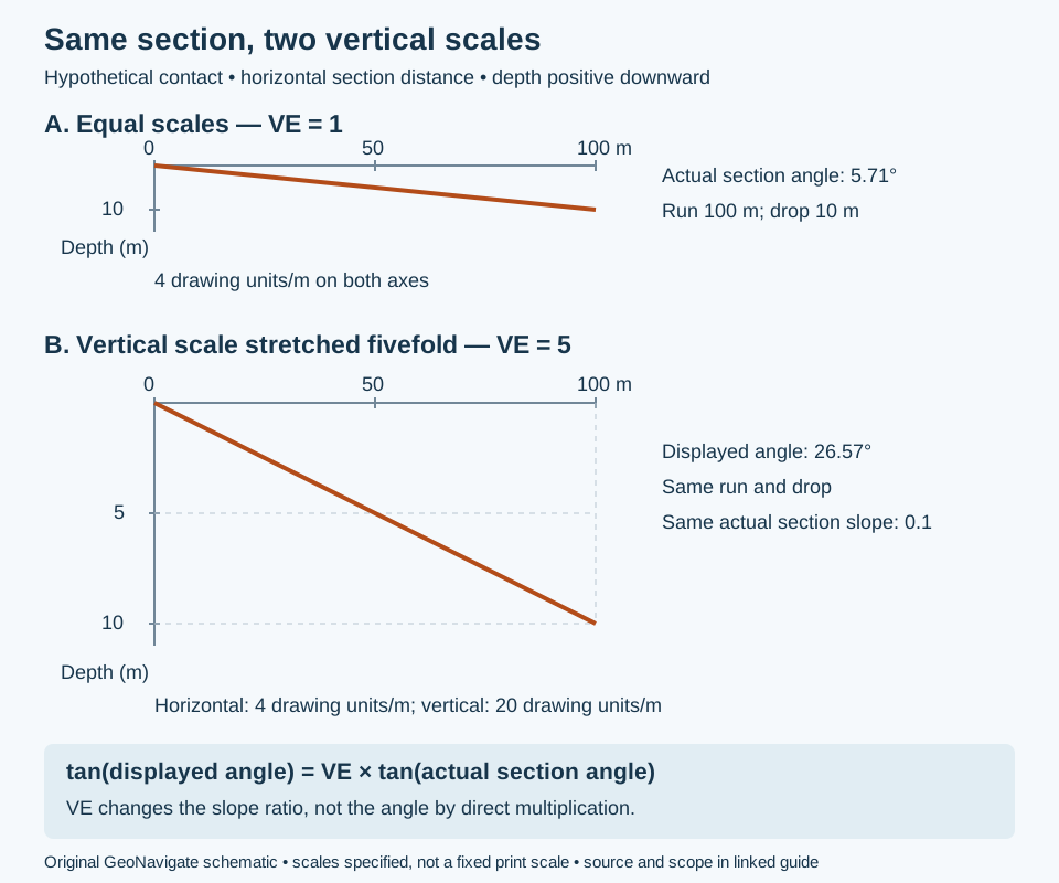
Consider an invented planar contact that drops 10 m over 100 m of horizontal distance along a fixed section heading. Depth is positive downward. Its actual section slope is 10/100 = 0.1 and its angle from horizontal is arctan(0.1) = 5.71°. These are section measurements; without the plane’s strike, they do not determine true dip.

Use slope ratios, not an angle multiplier

Let sₓ and s𝓏 be drawing length per metre horizontally and vertically, after converting both ground axes to metres. Then VE = s𝓏/sₓ. The displayed slope is (s𝓏 × Δz)/(sₓ × Δx), so:

tan β = VE × tan α, or α = arctan(tan β / VE), where α is the actual section angle and β the displayed angle.

1. With 4 drawing units per metre on both axes, VE = 1. The 100 m run occupies 400 units and the 10 m drop occupies 40 units.
2. Keep the horizontal scale and use 20 drawing units per vertical metre. VE = 20/4 = 5; the same drop occupies 200 units.
3. The displayed slope is 200/400 = 0.5, giving β = 26.57°. Multiplying the original angle by five would give 28.55°, which is incorrect.
4. Recover α using arctan(0.5/5) = 5.71°. Use unrounded values in calculations.

Interpretation checks

A change of section heading and a change of plotting scale are different operations. First remove scale distortion; then apply the apparent-dip projection if the plane orientation is known. The actual section angle equals true dip only along the dip direction. Measured depth along a curved well is not the horizontal distance used here. Different horizontal and vertical units, nonuniform image stretching or a varying axis scale require separate correction; one VE number cannot repair a nonuniform distortion.

Reference: Saunders, Welch and MacKinnon, Laboratory Manual for Introduction to Physical Geography, Lab 15, scale-ratio definition and profile interpretation, checked 31 October 2026. The section calculation and artwork above are original. Also see the Oilfield Glossary entry, Chaser Geological services and contact Chaser Geological.

Worked thickness example: a vertical interval is not normal thickness

Thickness needs a measurement direction. True stratigraphic thickness (TST) is perpendicular to bedding; true vertical thickness (TVT) joins parallel contacts vertically at one map location. Along-hole length follows the borehole. These quantities coincide only in particular geometries.

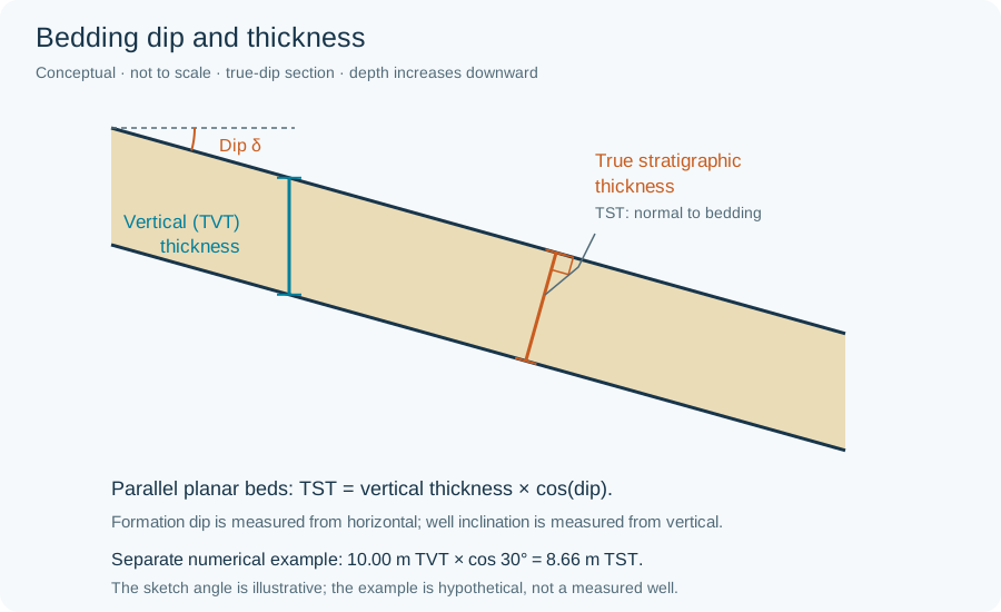
Assume two parallel planar contacts, true dip 30°, and a vertical top-to-base interval of 10.00 m. Projection onto the bedding normal gives TST = 10.00 × cos 30° = 8.66 m. Conversely, a bed with TST 10.00 m at the same dip has TVT 10.00 / cos 30° = 11.55 m. Swapping these two input thicknesses changes the question.

Applying the geometry to a drilled interval

For a straight trajectory crossing both parallel contacts once, let θ be the acute angle between the trajectory and the bedding normal. Then TST = along-hole length × cos θ. A hypothetical 20.00 m crossing at θ = 60° represents 10.00 m TST. θ is neither automatically well inclination nor formation dip: both trajectory azimuth and inclination matter. A path parallel to the bed does not cross its top and base in this planar model.

For a curved surveyed path through constant parallel planes, project the displacement between the two contact intersections onto the unit bedding normal: TST = |n · (r₂ − r₁)|. Do not substitute the measured-depth difference for that displacement. Coordinates must share a metric frame and vertical datum; choose one sign convention consistently. This vector expression is a geometric derivation, not an estimate of unobserved bed orientation.

Checks before interpreting a thickness change

• Confirm the same top and base are correlated, rather than a repeated fault slice or a different sandstone package.
• Use true dip, not the visually exaggerated angle on a plot or an oblique apparent dip.
• Check surveys and contact-depth uncertainty before interpreting apparent thickening as depositional change.
• Where contacts curve or are not parallel, use a local geological model; one cosine correction is insufficient.

These invented examples explain geometry, not steering instructions or measured reservoir thickness. Reference: University of Alberta, Geological Structures: a Practical Introduction — Primary Structures, thickness calculations. Continue with isopach and isochore mapping.

Isopach or isochore? Name the mapped quantity

An isopach joins equal true stratigraphic thickness; an isochore joins equal vertical thickness. A map title saying only “sand thickness” leaves this distinction unresolved. Also specify whether the interval is gross unit thickness or a net interval selected by stated criteria.

The schematic above identifies TVT vertically and TST normal to bedding. Consider two hypothetical local planar bed segments, each with 10.00 m TST. At location A the bed is horizontal, so TVT = 10.00 m. At B it dips 60°, so TVT = 10.00 / cos 60° = 20.00 m. Both locations have equal normal thickness, despite a twofold difference in vertical separation. These are local geometric examples, not a constructed regional fold model or evidence of sediment accumulation.

With depth positive down, subtract the top-surface depth from the base-surface depth at the same XY location to obtain TVT. A vertical difference between unrelated points, or a measured-depth interval in a deviated borehole, is not the same operation. Convert to TST only where the assumed bed orientation and geometry are supported. Near-vertical, overturned or fault-repeated sections need a model that resolves which contacts are paired; crossing surfaces must not be silently turned into positive thickness with an absolute value.

For a useful map legend, record the top/base definitions, units, datum, thickness direction, net/gross criteria, control locations and interpolation limits. A thickness contour is not a structure-depth contour, and neither proves reservoir connectivity. References: SLB Energy Glossary: isochore and isopach; geometry follows the university thickness reference above. No publication figure is reproduced.

Worked accounting example: qualify net-to-gross

A thickness map and a reservoir-quality classification answer different questions. Define the gross interval first, then identify which subintervals meet explicit criteria. Net-to-gross must name its numerator: net reservoir and net pay need not select the same rock.

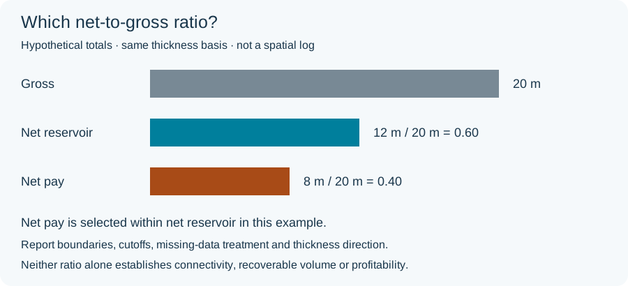
Assume a hypothetical 20 m gross interval on one stated thickness basis. A documented reservoir-quality screen retains 12 m; a further hydrocarbon screen retains 8 m within those 12 m. Net-reservoir/gross is 12/20 = 0.60 (60%), whereas net-pay/gross is 8/20 = 0.40 (40%). The ratio 8/12 ≈ 0.67 answers a third question: the selected pay fraction of net reservoir, not the net-pay fraction of gross.

If a revised, documented criterion retains only 6 m as pay, net-pay/gross becomes 0.30 while the gross interval remains 20 m. This is classification sensitivity, not physical thinning. The numbers are invented; no universal porosity, permeability or saturation cutoff is proposed.

Make the calculation reproducible

• State the top and base, depth datum and thickness direction; do not divide along-hole net by vertical gross.
• Apply flags to interval thicknesses, not simply to the number of log samples when sampling is uneven. Do not count overlapping qualifying intervals twice.
• Report gaps as unknown unless an explicit rule supports another treatment; missing data are not automatically nonreservoir.
• Separate interpreted pay from demonstrated flow and field economics. A ratio alone cannot establish connected volume or commercial production.

References: SLB: pay; P. F. Worthington, Net Pay (2010), DOI 10.2118/123561-PA (publisher summary); Dennis Denney’s JPT technical highlights (publisher-indexed excerpt). The full paid papers were not reviewed; no author figure is reproduced.

Fault separation versus slip: what does an offset actually constrain?

Fault separation measures an offset in a specified view. Net slip describes relative movement. Keeping those questions separate prevents an attractive correlation from becoming an unsupported movement history.

A fault-plane exercise with invented coordinates

Imagine looking straight at a planar fault, with both walls' marker traces overlaid. This is a view within the fault plane, not a vertical well section or a map. Let x increase along a stated strike direction and y increase down dip, both in metres. Assume rigid translation, no rotation and straight marker cutoffs. On reference wall A the bed cutoff is y = x; on wall B it is y = x + 4.

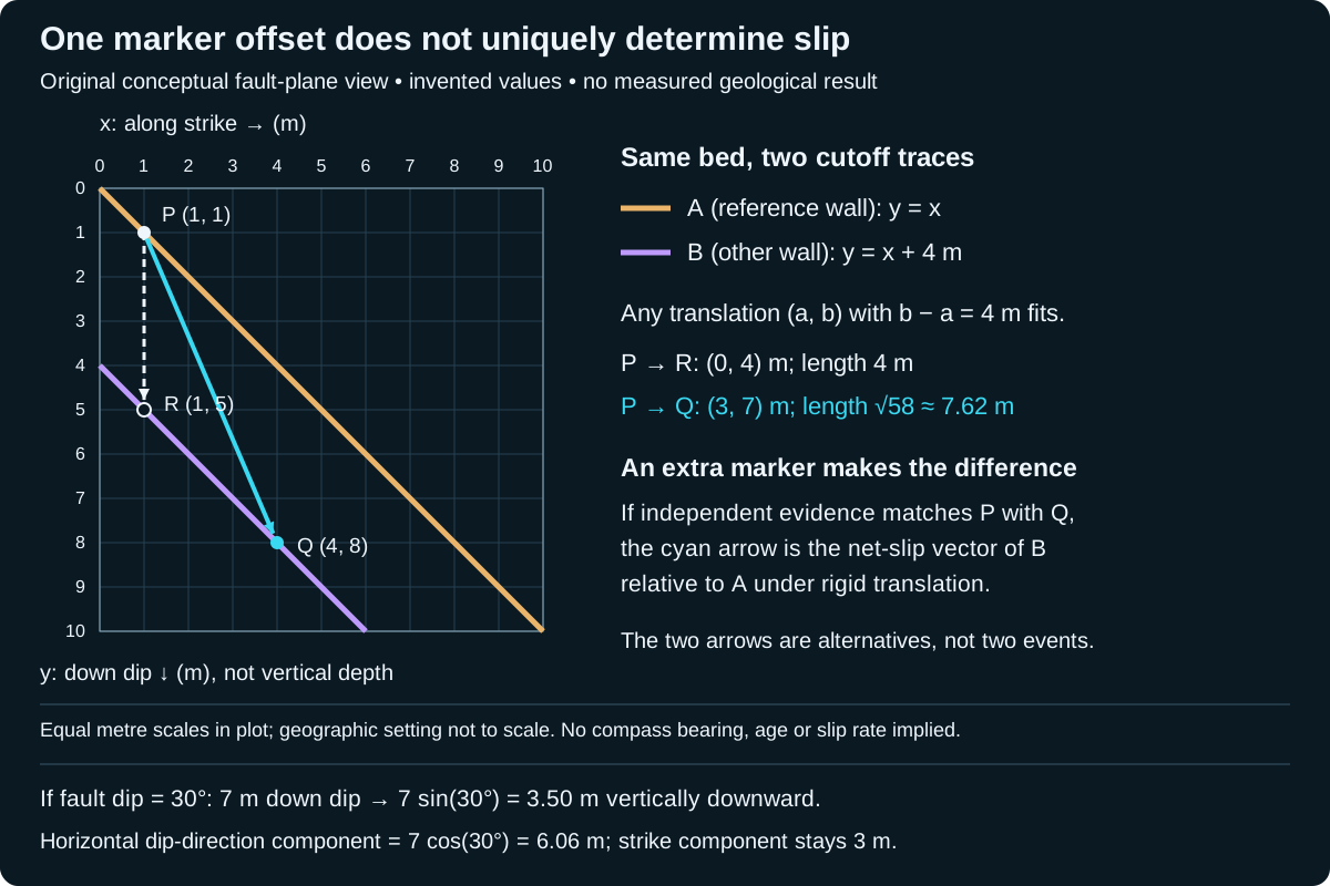
Translate any point (x, x) on A by a candidate vector (a, b). Its new coordinates are (x + a, x + b). To reach B, they must satisfy x + b = x + a + 4, so b − a = 4 m. This single equation permits many vectors.

• Candidate 1: (a, b) = (0, 4) m. Its length is 4 m.
• Candidate 2: (a, b) = (3, 7) m. Its length is √(3² + 7²) = √58 ≈ 7.62 m.
• Both shift A onto B. The 4 m dip-direction separation therefore does not, by itself, establish a 4 m net slip.

Add an independently matched piercing point

Suppose an independently correlated vein–bed intersection identifies P = (1, 1) m on A and Q = (4, 8) m on B as the two remnants of the same pre-fault feature. These are a matched piercing-point pair. Taking A as fixed, Q − P = (3, 7) m selects candidate 2. Its in-plane angle from positive x toward positive y is arctan(7/3) ≈ 66.8°. That is a stated rake convention, not a compass bearing or plunge. Reversing the reference wall reverses the vector.

The down-dip component is 7 m, not 7 m of vertical depth. A geographic reconstruction also needs the fault attitude. The calculation assumes the matching and rigid-translation model are valid; it cannot determine a movement date, rate, earthquake count or a history of reversals. A net vector does not reconstruct every step of a curved or reversing path.

From a correlation pick to a defensible interpretation

1. Label what was observed: marker identity, cutoff positions, view direction, coordinate reference and uncertainty. Do not silently replace a missing marker with a preferred correlation.
2. Test the correspondence with independent evidence. In this exercise, remove the vein constraint and P can correspond to many positions on B again.
3. Compare slickenlines and other movement indicators with the proposed vector. A line orientation alone normally leaves two possible senses; it does not supply a displacement length.
4. Check for curved faults, distributed deformation and multiple slip episodes before applying a one-plane translation. Different markers may record different histories.

For well correlation, report a formation-top mismatch in its actual depth/reference framework first. It does not automatically equal net slip on a fault. This example supplies a geometric test, not a wellsite fault diagnosis or a reservoir-connectivity prediction. Compare the separate Oilfield Glossary entry and the preceding orientation examples.

Project a known slip vector into geographic components

Continue the invented P-to-Q displacement above: 3 m along the chosen positive strike direction and 7 m down dip. Now stipulate that the planar fault dips 30° from horizontal. The strike direction is horizontal; the down-dip direction is inclined. This additional attitude is an assumption for this exercise, not information recoverable from the original fault-plane plot.

• Vertical downward component: 7 sin(30°) = 3.50 m.
• Horizontal component toward the dip azimuth: 7 cos(30°) = 6.06 m, rounded.
• Horizontal strike-parallel component: 3.00 m.
• Total horizontal magnitude: √(3² + 6.062²) ≈ 6.76 m; combining this with 3.50 m vertical recovers the original net length √58 ≈ 7.62 m.

The horizontal components are perpendicular and must be combined as vectors, not added as 3 + 6.06. A compass bearing still requires the chosen strike direction and dip azimuth. Reversing the reference wall reverses all component signs, while leaving the net magnitude unchanged. This is a coordinate projection of a stipulated displacement, not a new estimate of slip from bed separation.

For a well interpretation, keep a depth mismatch, an apparent marker separation and a reconstructed slip vector as separate records. A vertical top offset alone does not supply the two in-plane components used here. Curved faults or distributed strain also fall outside this rigid planar model. The extended full-size schematic labels the projection assumptions without changing its original fault-plane axes.

Original calculation checked 29 October 2026. Component terminology was checked against primary-source indexed text from University of Michigan, Faults and ETH Zürich, Faults and Joints; direct full-page retrieval was unavailable this pass. No measured displacement, private well data or external expert review is claimed. Compare oilfield fault separation and Chaser interpretation services.

References and scope

• Waldron and Snyder, University of Alberta: Faults — separation, cutoff geometry and piercing-point constraints.
• University of Michigan, Physical Structural Geology and Tectonics: Faults — net-slip vector, components and reference-wall sense.

Original explanation, calculation and vector artwork; sources checked 27 October 2026. No expert review claimed. Explore geology guides, Chaser Geological services or contact GeoNavigate.

Worked fabric example: rock cleavage and crenulation

A split face is a starting observation, not a complete structural interpretation. Rock cleavage describes repeated rock-scale planes of weakness. Mineral cleavage describes breakage within a crystal. Record which object is splitting before using the word “cleavage” in a core log.

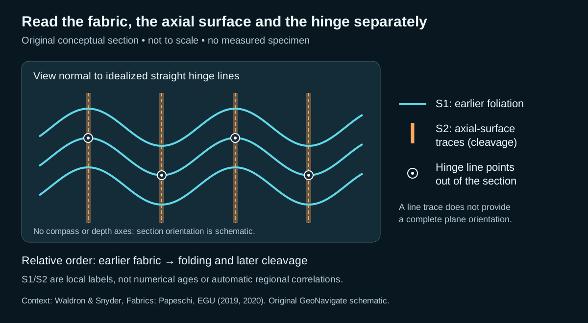
Hypothetical specimen: three features, three records

Invented observations; no private sample or well data

Observation	Record	What remains uncertain
A mica-rich fabric can be followed continuously around small folds.	Earlier foliation, locally labelled S1.	Its age, original orientation and regional correlation.
A repeated planar fabric follows the axial surfaces of those folds.	Candidate crenulation cleavage, locally labelled S2.	Whether the apparent alignment persists in adjacent sections.
The fold hinges form parallel ridges on an exposed fabric surface.	Crenulation lineation.	Trend and plunge until the specimen is oriented.

The supported sequence is earlier fabric → folding and later cleavage. It does not require a dated interval between events. S1/S2 labels are a local bookkeeping convention here: do not correlate them automatically with labels in another outcrop or well.

Check the geometry before reporting an orientation

In the drawing, a hinge line is perpendicular to the section and therefore appears as a dot. The orange line is the intersection of an axial surface with the section; it is not itself the full surface. A measured angle between two traces on an unoriented slab cannot supply strike, dip, trend or plunge. Keep the slab orientation and viewing direction with the photograph, then measure planes and lines using their respective conventions.

For a wellsite note, separate visible mineral alignment, fold geometry, splitting behaviour and inferred sequence. Examine another face or an oriented thin section to test continuity. Small detached cuttings may retain a fabric but lose the orientation and cross-cutting context needed to establish the sequence. Avoid turning one fabric into a unique stress direction or a regional tectonic history.

References checked 27 October 2026: Samuele Papeschi, EGU Foliation (2019) and Crenulation cleavage (2020); Waldron and Snyder, Fabrics (definition verified in indexed university text; direct page fetch unavailable). Original teaching case; no expert review or reproduced photographs claimed. Continue to the Oilfield Glossary or contact Chaser Geological.

Worked example: which way is stratigraphic up?

Imagine three beds with independently established depositional ages of 120, 110 and 100 Ma. In an upright horizontal stack, walking upward through them encounters progressively smaller ages: 120 → 110 → 100 Ma. In the completely overturned horizontal end member, the same younging order runs downward. The age difference between the outer beds remains 20 million years; turning the rocks changes their orientation, not their depositional sequence. These ages are invented and assume the dates constrain deposition rather than inherited grains.

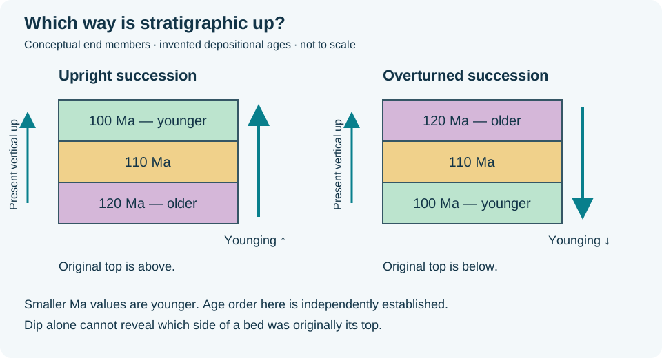
In the field, dates may be unavailable. Look for consistent primary structures that establish younging direction. A bed reliably interpreted as normally graded fines toward its original top. If that top points downward today, it supports overturned bedding. First distinguish normal grading from inverse grading, alteration and sampling artefacts; corroborate it with other way-up indicators or mapped age relations. Unoriented cuttings do not retain the bed's spatial orientation.

For a wellsite correlation, record “dip measured; younging unresolved” when orientation evidence is missing. Repeated gamma-ray shapes or increasing measured depth alone cannot prove a reversed stratigraphic succession. A single overturned limb also does not determine the facing of the whole fold: fold facing is younging within the axial surface, perpendicular to its hinge. It needs the fold geometry as well as the bed-age evidence.

Concept references: Waldron and Snyder, Primary Structures; Folds; Earle, Folding.

Worked example: two limbs make a fold profile

A section that cuts across a fold can contain several local dips. Consider an invented cylindrical fold with a horizontal north–south axis, viewed in a vertical west–east profile perpendicular to that axis. Its straight west limb dips 30° east and its east limb dips 50° west. Both descend toward the hinge, so this is a synform. The drawing represents one folded surface, not a topographic valley or a pair of faults.

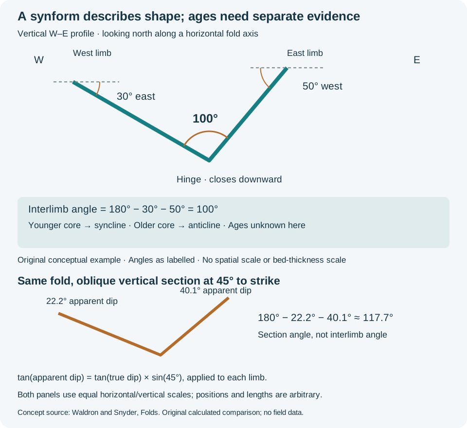
For these opposite-facing, non-overturned limbs in a true vertical profile, the interlimb angle is 180° − 30° − 50° = 100°. The subtraction follows from the triangle formed by the limb traces and a horizontal line above the hinge. The University of Alberta chapter's Davis et al. scheme calls this open. Class boundaries differ among schemes, so retain the numerical angle and the cited scheme in the description.

This shortcut is conditional. Do not apply it unchanged to overturned limbs, an oblique section or a plunging axis. For a cylindrical fold, construct the profile perpendicular to the axis; a profile of a plunging fold is not generally vertical. On rounded folds, specify where the limb tangents were measured. A local dip near the hinge is not a substitute for a representative limb measurement. The apparent-dip projection above explains why an oblique vertical view of this horizontal-axis example would distort its limb angles.

Worked check: apparent fold opening

Keep the same horizontal-axis fold, but cut a vertical section trending 045°, at 45° to the north–south strike of both straight limbs. Applying tan(apparent dip) = tan(true dip) × sin(45°) gives 22.2° and 40.1°. The angle between those section traces is approximately 117.7°, compared with 100° in the true profile. The rock did not unfold: only the section direction changed. These rounded values are calculated from the original 30° and 50° inputs.

In a well-path section, record the section bearing before comparing apparent opening with a mapped fold profile. This two-limb calculation assumes the stated cylindrical, horizontal-axis geometry; it is not a correction for every plunging or non-cylindrical fold. The lower SVG panel shows the calculated traces at equal horizontal and vertical scales.

What age evidence would change the name?

Geometry alone leaves the age classification unresolved. If independent stratigraphic evidence establishes younger beds in the core, describe a synformal syncline. If it establishes older beds in the core, the same downward-closing shape is a synformal anticline. An antiform is the upward-closing shape and likewise does not, by itself, establish age order.

For a wellsite handover, keep observations and interpretation in separate sentences: “Opposing limb dips define a downward-closing profile; relative ages remain unresolved.” Then list the evidence still needed, such as mapped unit succession, fossils or reliable sedimentary way-up indicators. Repeated gamma-ray motifs alone do not establish stratigraphic younging, and a folded reservoir is not automatically a sealed trap. Carry both the geometry and its uncertainty into the correlation.

Concept references: Earle, Physical Geology 2e, Folding; Waldron and Snyder, Folds; Introduction to Folds, Lab 4. Original calculation and artwork; no publication figure, field measurement or expert review is claimed.

Worked example: separate lineation mechanisms before correlating them

A lineation is a penetrative or repeated linear fabric; it is not one genetic feature. The first task is to name what defines the line. An intersection lineation is common to two identified planes, a crenulation lineation follows aligned hinges of small folds in an earlier foliation, and a stretching lineation is carried by elongate minerals, clasts or aggregates.

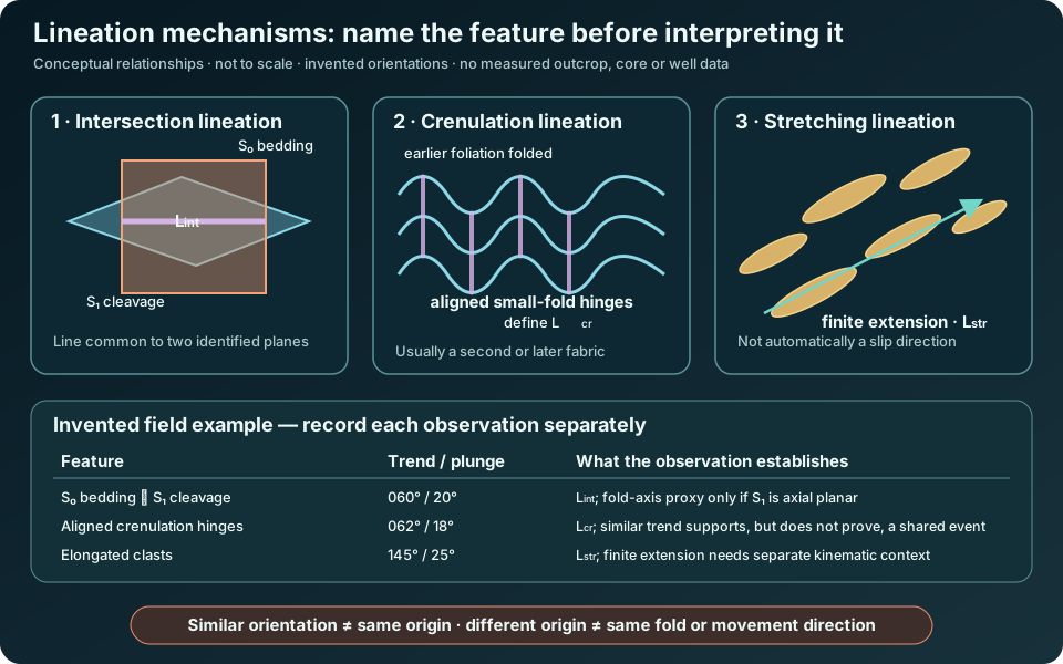
In the invented example, the bedding–cleavage intersection trends and plunges 060°/20°, while the crenulation hinges are 062°/18°. Their near-parallel orientations could support a shared cylindrical fold-axis interpretation if field relations establish that the cleavage is axial planar and that the crenulations belong to the same deformation. Similar numbers alone do not prove that history. The elongated clasts define a separate stretching lineation at 145°/25°; this records a finite-extension direction, not automatically the slip direction or transport sense.

Record observations before assigning kinematics

1. Identify the material feature: two intersecting surfaces, small-fold hinges, elongate objects or another repeated line.
2. Measure trend and plunge, state the north reference, and record the supporting planes or host foliation. An intersection line is only reproducible when both planes are known.
3. Establish overprinting order. A crenulation folds an earlier fabric, so it cannot be interpreted without naming that older fabric.
4. Keep the measured line separate from inferred fold axis, extension direction and movement sense. Test each interpretation against independent geometry and kinematic indicators.

For wellsite work, unoriented cuttings generally do not preserve a defensible trend and plunge. Oriented core, borehole-image data or another referenced orientation method is needed before a linear fabric can be placed in geographic coordinates. A repeated linear texture in a sample can still be described, but its spatial orientation and structural meaning should remain unresolved.

Concept reference: Waldron and Snyder, Fabrics, and University of Potsdam, DIoGeneS structural-elements key. For orientation conventions, see Earle, Measuring Geological Structures. Original explanation, example and artwork; no publication figure, measured dataset or expert review is claimed.

Worked example: trend, plunge and rake

Describe a line with trend and plunge, and state the order explicitly. In this invented example, trend/plunge = 030°/20° means the line slopes downward toward azimuth 030°, at 20° below horizontal. Trend is measured clockwise from the stated north reference in plan; plunge is measured in a vertical section along that trend. Neither arrow establishes movement sense.

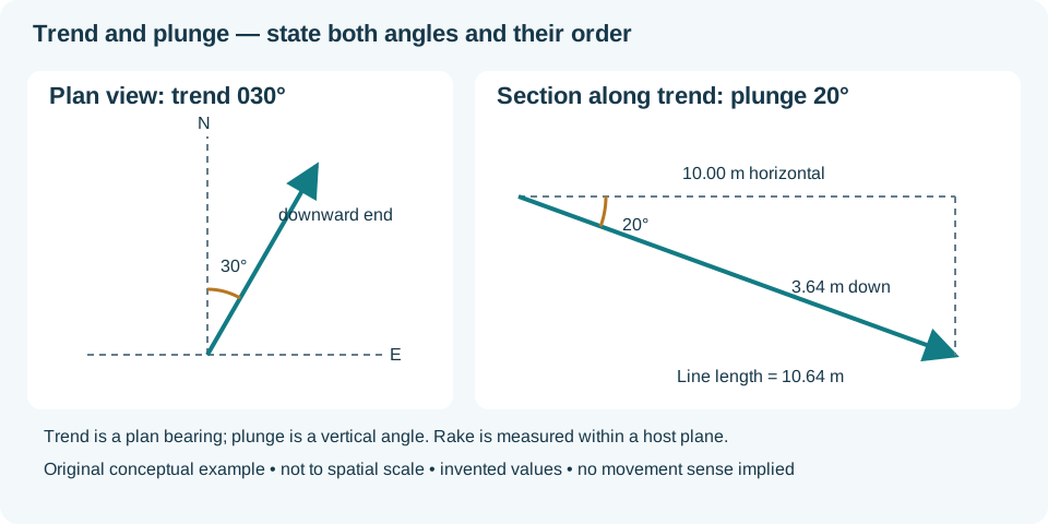
For 10.00 m of horizontal distance along the trend, the downward change is 10.00 × tan(20°) = 3.64 m. The distance along the inclined line is 10.00 / cos(20°) = 10.64 m. These distances are different quantities; a vertical section in another azimuth would not show the same slope.

Rake is measured in the host plane

Rake (pitch) measures from a specified strike end within the plane carrying the line. Consider a separate invented plane with right-hand-rule strike/dip 000°/30° (dipping east). A line with a 45° rake measured from north toward down-dip has north, east and downward unit-vector components cos45°, sin45° cos30° and sin45° sin30°. Its trend is atan2(east, north) = 040.9°, and its plunge is asin(down) = 20.7°. The 45° rake is therefore not a 45° plunge.

Record the host plane, reference strike end, north reference and angle convention. A horizontal unoriented line has two equivalent opposite bearings; a vertical line has undefined trend. Check that a line lying in a plane has plunge no greater than the plane dip. Oriented core or referenced borehole images may support these measurements; unoriented cuttings generally cannot. See the oilfield rake entry for the same convention warning.

Concept references: Géologie Québec, Structural Measurements and Waldron and Snyder, Orientation of Structures. Examples and artwork are original; no field result or expert review is claimed.

Field guide: fault core, damage zone and slickenlines

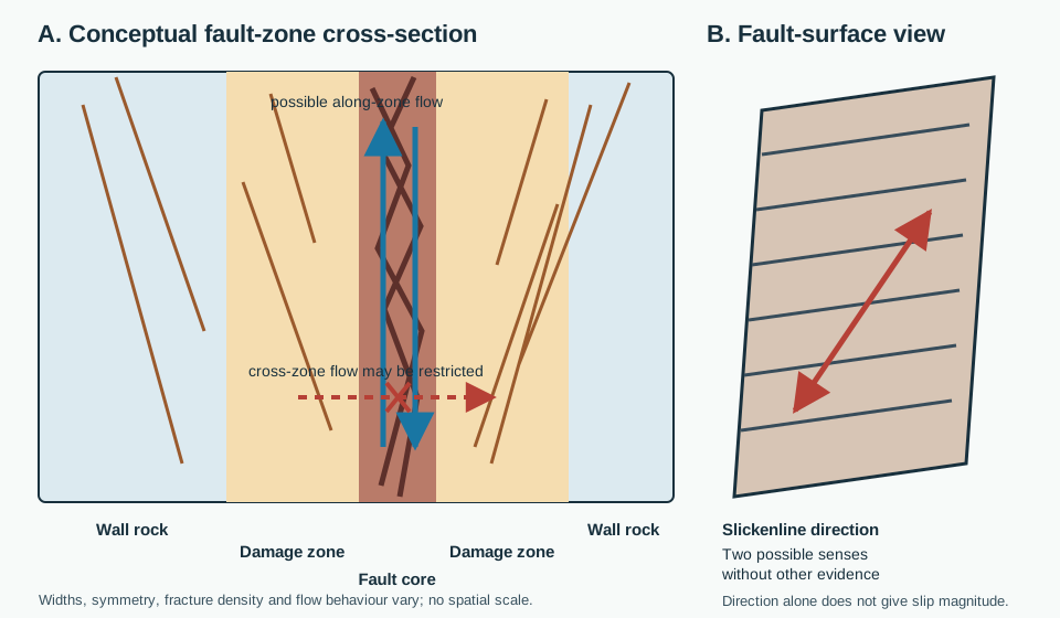
A mapped fault is often a zone rather than one clean plane. Start with description: locate any fault core, then describe the surrounding damage zone and less-deformed wall rock separately. Core rock has been reworked enough that original neighbours may no longer fit together; damaged wall rock retains recognizable earlier relationships despite fractures, veins, small faults or folds.

Keep rock name, architecture and hydraulic behaviour separate

Fault gouge is fine-grained broken material without primary cohesion; cataclasite is cohesive rock dominated by brittle fragmentation and grain-size reduction. Either observation helps describe the core, but neither makes the entire fault a universal seal or conduit. A clay-rich continuous core may restrict cross-fault flow while connected fractures may enhance flow parallel to the zone. Mineralogy, stress, cement, aperture, continuity and scale still need evidence.

Direction is not sense or distance

A slickenside is the smoothed or polished movement surface. Its linear scratches, grooves or mineral fibres are slickenlines. Their trend/plunge or rake constrains a line of slip in the fault plane, but that line has two opposed senses. Assign normal, reverse, dextral or sinistral movement only when independent asymmetric indicators, offsets or matched piercing points support it. One offset marker gives separation in the view measured; it does not by itself recover the three-dimensional slip vector.

In core or image logs, first preserve orientation confidence and distinguish a true fault surface from drilling-induced scratches. Record sample scale and the interval over which fracture intensity changes. Unoriented cuttings can support a fault-rock description, but generally cannot establish geographic slickenline attitude or fault-slip sense.

Concept references: Waldron and Snyder, Faults; BGS fault-gouge classification; and BGS cataclastic-rock classification. Text and artwork are original; no site measurement, reproduced figure or expert review is claimed.

Worked example: joint sets and fracture aperture

A joint set groups similarly oriented joints; it does not describe the width of their openings. In an invented mapping exercise, six near-vertical joints strike 028–034° and five strike 118–124°, with bearings referenced to true north. Report two orientation groups and their observed spread. A plan sketch alone cannot establish when each group formed, how far its fractures extend, or whether their intersections transmit water.

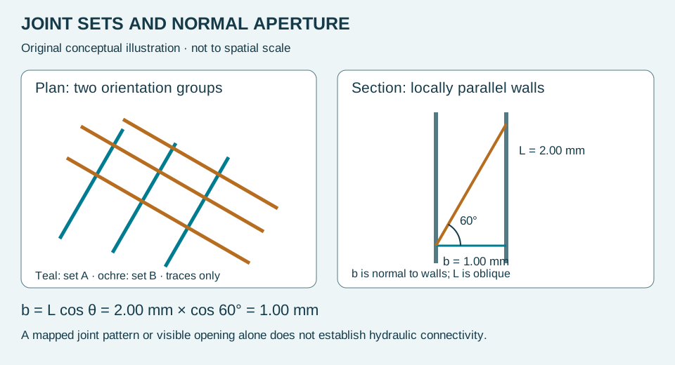
Now measure the opening between two locally parallel walls. Let L be an oblique wall-to-wall segment and theta its angle from the wall normal. Its normal projection is b = L cos theta. For an invented L = 2.00 mm and theta = 60°, normal aperture b = 1.00 mm. At theta = 0°, L equals b. A line parallel to the walls cannot cross the opening, so the 90° limit is not a valid wall-to-wall measurement.

This calculation assumes the measured segment and wall normal lie in the illustrated plane and the walls are locally parallel. Rough, curved or contacting walls require local measurements with stated directions. Record mineral fill separately from remaining void space. Core recovery, unloading and handling can change openings; unoriented cuttings cannot supply a geographical joint-set orientation. Use the geological-joint entry to distinguish natural structure from pipe terminology and drilling breaks.

References: Waldron and Snyder, Fractures (joint geometry and aperture); Panchuk, Fractures, Joints, and Faults (joint sets). The projection example and drawing are original teaching material.

Worked example: mineral fill versus open aperture

A mineral vein and an open fracture describe different properties: mineral fill versus remaining space. Crack-seal growth describes repeated opening and sealing. Keep these observations separate when describing core or an outcrop.

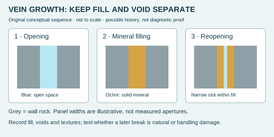
In an invented ideal section, parallel wall-rock boundaries are 3.0 mm apart. Solid mineral fill occupies 2.6 mm of the normal traverse and one continuous open slot occupies 0.4 mm. The check is 2.6 + 0.4 = 3.0 mm. Report both the wall-rock separation and the remaining open slot; calling the entire 3.0 mm an open aperture would overstate the observed void. This balance assumes nonoverlapping fill and void segments measured along the same wall-normal line.

A neighbouring section may be completely filled or have a different opening. Neither this local balance nor the diagram establishes a connected flow path. Before interpreting the slot as natural reopening, examine whether it cuts mineral grains or follows grain boundaries, compare adjacent intact material, and consider drilling and handling damage. Preserve the observation separately from the proposed history.

For an idealised growth exercise, three independently established opening increments of 0.10, 0.20 and 0.10 mm sum to 0.40 mm of cumulative opening if there is no dissolution, closure or shear. This is not a method for converting three visible colour bands into three events. A final thickness supplies neither elapsed time nor a growth rate. Compare the aperture definition and the preceding normal-projection example.

Concept reference: Waldron and Snyder, Fractures — features of vein fills. Calculations, teaching scenario and artwork are original GeoNavigate material; no expert review is claimed.

Field guide: ductile shear zones and mylonitic fabrics

A ductile shear zone concentrates continuous deformation across a zone rather than on one through-going brittle fracture. At depth, it may connect with a surface fault; later cooling can add fractures, gouge or cataclasite. Describe the observed rock and overprints before assigning one mechanism to the entire history.

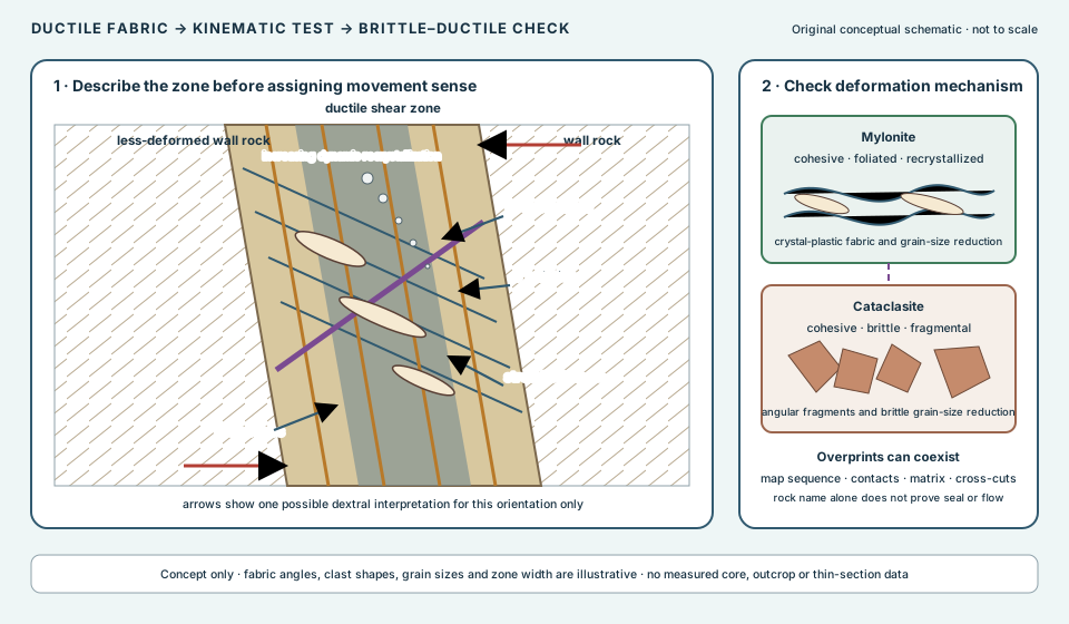
Separate observation from kinematic interpretation

1. Orient the sample or exposure. Record strike, dip, top/underside and viewing direction. A mirror view can reverse an apparent sense indicator.
2. Describe the fabrics. In an S–C fabric, S is the more oblique penetrative foliation; C surfaces are closer to the shear-zone boundary and commonly host stronger deformation.
3. Identify cross-cutting bands. A C′ shear band cuts and offsets the older foliation. Confirm displacement rather than relying on one dark line.
4. Check the matrix. Mylonite records crystal-plastic deformation and dynamic recrystallization. Angular fragments in a brittle matrix instead support cataclasis, though both may coexist or overprint one another.
5. Combine indicators. Use asymmetric porphyroclasts, mineral fish, deflected foliation, shear bands and stretching lineation together. One ambiguous indicator does not establish regional transport.

Invented strain-gradient exercise

Across a hypothetical 12 m traverse normal to a shear zone, six equal 2 m intervals are described only by the fraction of the original coarse grains that remains visible: 80%, 60%, 40%, 20%, 10% and 5%. These observations show an inward decrease in preserved coarse grains, but they are not a linear strain gauge. The arithmetic mean is (80 + 60 + 40 + 20 + 10 + 5) / 6 = 35.8%, rounded; it does not mean the zone has “64.2% shear strain.” Grain survival depends on mineral, temperature, fluid, deformation mechanism and section orientation. Map the gradient and test microstructures rather than converting the percentage directly to displacement.

In wellsite work, unoriented cuttings may reveal foliated or recrystallized rock but cannot preserve reliable shear-sense geometry. Oriented core and thin sections are required for directional fabric interpretation. A mylonitic interval also does not, by name alone, establish present permeability or fault seal.

Concept references: Waldron and Snyder, Shear Zones; Panchuk, Dynamic Metamorphism; and the British Geological Survey Moine framework. The exercise and artwork are original GeoNavigate material; no expert review is claimed.

Thin-section guide: porphyroclasts and recrystallization

A large crystal in a fine matrix does not have one automatic origin. A porphyroblast became conspicuous through metamorphic growth. A porphyroclast is a relict grain left conspicuous because deformation reduced the grain size around it. Preserve that process distinction in core and thin-section descriptions.

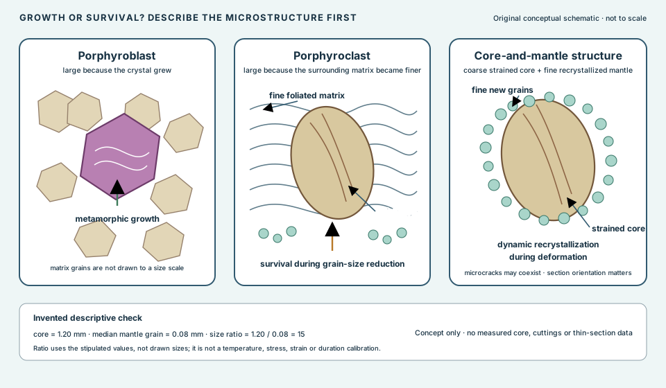
Observation sequence

1. Identify the coarse grain. Record mineral, boundaries, inclusions, fractures, undulose extinction, twins and subgrains.
2. Describe the matrix independently. Note grain size, foliation, ribbons and whether new grains occur along the coarse grain boundary.
3. Test the relationship. A relatively coarse strained core surrounded by finer recrystallized grains is a core-and-mantle structure. It supports grain-size reduction around a relict core; it is not itself a thermometer or strain gauge.
4. Name the process cautiously. Dynamic recrystallization happens during deformation. Crystal-plastic deformation may also produce subgrains, twins and undulose extinction. Microcracks can coexist, so “ductile” and “brittle” observations should not be forced into separate samples.
5. Orient before interpreting asymmetry. Porphyroclast tails can support shear sense only in a suitable section with known orientation and independent indicators. A mirrored or oblique view can mislead.

A relict grain need not remain unchanged. BGS describes porphyroclasts becoming smaller by fracture or marginal erosion while the matrix develops around them. Thus a fractured coarse grain can still be a porphyroclast; large size alone does not establish metamorphic growth.

Invented grain-size check

Suppose a teaching thin section has a 1.20 mm relict core and a median recrystallized mantle grain size of 0.08 mm. The core-to-mantle ratio is 1.20 / 0.08 = 15. This ratio uses the stipulated dimensions, not measurements of the not-to-scale drawing. It does not yield temperature, differential stress, shear strain or duration without mineral-specific calibration, uncertainty and a justified deformation mechanism.

In wellsite work, cuttings may contain recrystallized fragments yet lose their original orientation and zone context. Log the texture and uncertainty; reserve kinematic interpretation for oriented core, image logs or properly oriented thin sections. No present-day permeability or seal behaviour follows from the microstructure name alone.

Concept references: Waldron and Snyder, Shear Zones; the British Geological Survey mylonitic-rock classification; and Ocean Drilling Program Leg 176 structural geology. The example and artwork are original GeoNavigate material; no expert review is claimed.

Worked example: classify the rock and retain uncertainty

Once deformation textures establish a mylonitic rock, the proportion of surviving porphyroclasts helps refine its name. Under the BGS scheme, protomylonite retains more than 50% by volume and ultramylonite retains less than 10%. State the scheme used, because descriptive names must travel with their criteria.

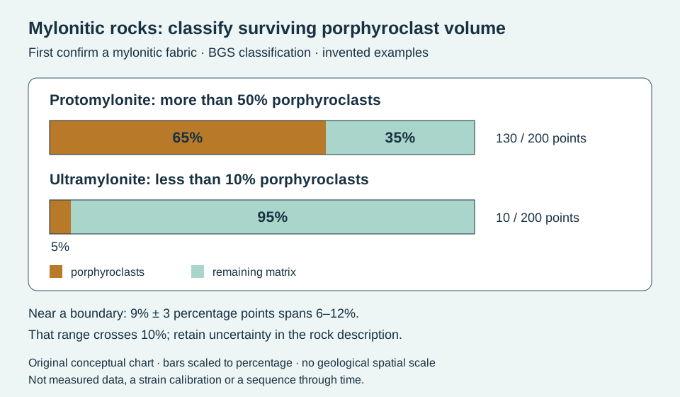
For an invented representative point count, 130 of 200 points fall on porphyroclasts: 130 / 200 × 100 = 65%. A second count yields 10 / 200 × 100 = 5%. These examples fall comfortably within the two end-member categories. Point counts estimate sectional area proportions; interpreting them as volume proportions requires representative sampling and appropriate section selection. They are not a count of individual grains.

A third sample is estimated at 9% with an illustrative uncertainty of ±3 percentage points. Its plausible range is 6–12%, crossing the 10% boundary. Report that uncertainty and the mylonitic fabric instead of presenting an unqualified ultramylonite assignment. The ±3 value is supplied for this exercise, not calculated from the first two point counts. At exactly 10%, the strict “less than 10%” criterion is not satisfied; at exactly 50%, “more than 50%” is not satisfied.

Inspect several representative fields, retain sample orientation and record how altered or ambiguous grains were handled. Fine matrix abundance alone cannot distinguish dynamic recrystallization from brittle fragmentation. A classification percentage also supplies neither displacement nor strain, and these three samples do not define successive stages in one deformation history. Compare the microstructure workflow and cataclasite.

Classification references: BGS PROMYL record and BGS ULMYL record. Original GeoNavigate examples and artwork; no expert review is claimed.

Finite strain: the same shape ratio can hide different area changes

When an elongated object appears in a thin section, first distinguish its observed shape from a reconstructed deformation. Finite strain compares an initial configuration with a final one. A strain ellipse represents the result for an initially circular marker under homogeneous deformation. Neither term makes an unknown original grain shape known.

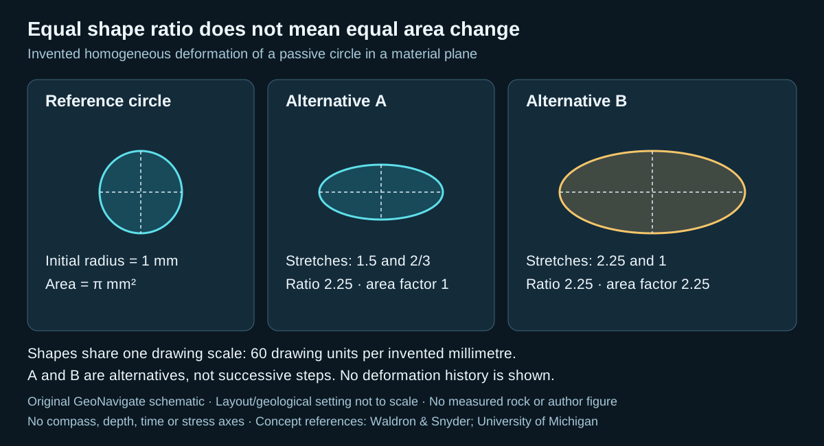
Worked example: start with a known circle

Assume a passive circular marker with initial radius 1 mm, uniform deformation within its material plane, and perpendicular principal directions. The invented numbers below are exact for the exercise. Stretch is final length divided by initial length; extension is stretch minus one. Both are dimensionless.

• Case A: principal stretches are 1.5 and 2/3. The final semiaxes are 1.5 mm and 2/3 mm. The major-to-minor ratio is 1.5 ÷ (2/3) = 2.25.
• Case B: stretches are 2.25 and 1. The final semiaxes are 2.25 mm and 1 mm. Its ratio is also 2.25.

For an ellipse of semiaxes a and b, area is πab. Dividing by the original area π × 1² gives area factors of 1 for A and 2.25 for B. A preserves area; B increases it by 125%. B's semiaxes are each 1.5 times A's, so its area is 1.5² = 2.25 times A's. Photographs resized until both ellipses have the same width would conceal that difference unless their scale information were retained.

In A, the long-axis extension is +0.5, or +50%; the short-axis extension is −1/3, or about −33.3%. Equal area does not require equal and opposite percentage extensions. Multiplying the stretches gives the area factor; adding the percentages does not. In B, the extensions are +125% and 0%.

What the calculation cannot supply

These are area changes within the specified plane. To turn them into volume changes, an additional out-of-plane stretch is required. If that stretch is stipulated to be 1, the volume factors equal the area factors; that is an extra assumption, not something a photograph proves.

Nor does either final ellipse reveal a unique deformation path. Even along a fixed direction, successive stretches of 1.2 and 1.25 multiply to 1.5; adding their 20% and 25% extensions would incorrectly give 45% instead of 50%. The elapsed time is absent, so this exercise supplies no strain rate. It also supplies no constitutive model or loading measurement from which to calculate stress.

Use with real rock descriptions

Record the section orientation, image scale, marker type and evidence for its initial shape before reporting a strain estimate. Compare several markers and describe variation rather than imposing uniform deformation on a visibly heterogeneous sample. Keep the measured outline separate from the interpretation that it represents a passive marker. A stretching lineation provides useful fabric context, while crystal-plastic microstructures address deformation mechanisms; neither automatically supplies all the missing reference dimensions.

Sources and scope

Concept references: Waldron and Snyder, Kinematic Analysis and Strain, for stretch and ellipse conventions; University of Michigan, Deformation and Strain, for finite strain, path dependence and marker interpretation. Original GeoNavigate prose, calculations and SVG; sources checked 27 October 2026. No private well data, reproduced artwork or external expert-review claim. Explore the Oilfield Glossary, Geology Guides, Chaser Geological services, or contact Chaser Geological.

Folding: separate layer geometry from evidence of slip

A curved bed describes a shape. Explaining how that shape developed requires additional evidence. Flexural slip concentrates relative movement on discrete layer-parallel surfaces; flexural flow distributes layer-parallel shear within the rock. These are end-member descriptions and can operate together or at different stages.

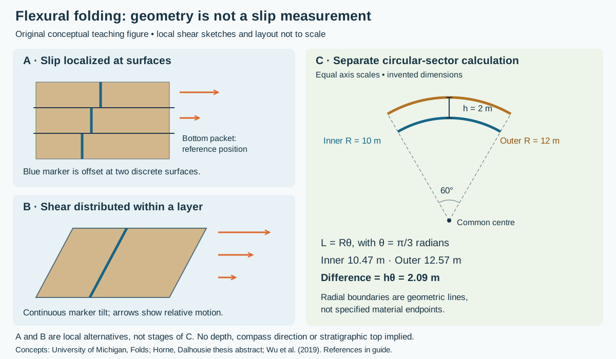
Worked geometry: why nested arcs have different lengths

Draw two concentric circular arcs between the same radial boundaries. Set inner radius R = 10 m, radial separation h = 2 m, and included angle θ = 60° = π/3 radians. Here h is the normal separation of the arcs, not vertical thickness. The angle is the sector angle, not an interlimb angle or a well inclination.

1. The inner arc length is Rθ = 10 × π/3 = 10.47 m, rounded.
2. The outer arc length is (R + h)θ = 12 × π/3 = 12.57 m.
3. The difference is hθ = 2 × π/3 = 2.09 m. Compute the difference before rounding.

Doubling the separation to 4 m at the same angle doubles the difference to 4.19 m. Halving the angle to 30° at the original 2 m separation halves it to 1.05 m. Arc-length arithmetic uses radians; entering 60 directly would give a result too large by 180/π.

Why 2.09 m is not automatically bedding slip

The calculation compares lengths between geometric radial lines. It does not identify the same material endpoints before and after deformation. To convert the mismatch into relative displacement, one would have to specify initial lengths, internal stretching or shortening, anchoring conditions and how material passes across each boundary. If those constraints are unknown, the number is a geometric difference only. Do not assign it to one fault, divide it between two limbs without a model, or use it as a displacement measured from a well log.

The local marker panels illustrate a different observation: discrete offsets across surfaces versus a continuous change in marker position through a sheared layer. They are not a time sequence, and their arrows are not inferred from the circular sector. Neither panel alone reconstructs the deformation of an entire fold.

Build a field interpretation from independent observations

• Describe hinges, limbs, bed thickness and section orientation before naming a mechanism. An oblique exposure changes the apparent geometry.
• Seek markers that cross suspected movement surfaces. Record their offsets and the reference frame; distinguish a displaced marker from a vein that grew along the surface.
• Compare movement indicators with bedding and hinge orientations on both limbs. Allow for changes along strike, later reactivation and internal strain.
• Keep fold interpretation separate from operational estimates of pore pressure, rock strength and permeability. This example supplies none of those measurements.

Research context and regional relevance

Horne's Dalhousie thesis abstract describes a Nova Scotia example with an early flexural-flow stage and later slip surfaces, linked ramps and veins. It illustrates why one fold need not have one mechanism throughout its history. Wu and colleagues' numerical study investigates how layering, friction and model conditions affect slip initiation; its specific thresholds should not be transferred directly to an Alberta well.

For southern Alberta context, the published Livingstone Range study documents flexural-slip thrust-propagation folds and changes along strike. That is a regional comparison, not evidence that every Deep Basin or Foothills structure follows the same geometry. A drilling correlation should test alternative structural interpretations using available observations, with formation identity and fault repetition kept explicit.

Sources and scope

• University of Michigan, Processes in Structural Geology and Tectonics: Folds — kinematic models; indexed primary text checked.
• Richard Horne, An Evaluation of Flexural-Slip Folding in the Meguma Group — Dalhousie thesis abstract, not a full-thesis review.
• Wu, Eckert, Liu and Obrist-Farner (2019), The Role of Flexural Slip during the Development of Multilayer Chevron Folds — university record and abstract, DOI 10.1016/j.tecto.2019.01.008.
• Along-strike variations and internal details of chevron-style, flexural-slip thrust-propagation folds within the southern Livingstone Range anticlinorium (2011) — publisher-indexed abstract checked; full article not reviewed.

Sources checked 27 October 2026. Original explanation, arithmetic and artwork; no private well data or reproduced publication figures. Explore the Oilfield Glossary, Geology Guides, Chaser Geological services, or contact Chaser Geological.

References and scope

Original GeoNavigate explanation, calculation and vector artwork, based on the public references below. The numbers describe an invented teaching plane. They are not a well dataset or a reproduced publication figure.

• Steven Earle, Physical Geology, 2nd edition: measuring geological structures — strike and dip.
• University of Alberta: Orientation of structures — bearings and recording conventions.
• Géologie Québec: Structural measurements on outcrops — Canadian right-hand rule.
• Lisle and Leyshon, Apparent dip (2004), DOI 10.1017/CBO9781139171366.016 — section orientation and apparent dip.

Explore the Geology Dictionary, Chaser’s wellsite geology services, or contact Chaser Geological.