
GEONAVIGATE / RESOURCES / HYDROGEOLOGY
Permeability versus hydraulic conductivity: worked examples
Compare permeability and conductivity, calculate a viscosity change, and work through groundwater flow along and across layered rocks.
Use one consistent equation
K = kρg/μ, where ρ is density, g gravitational acceleration and μ dynamic viscosity. This comparison assumes an unchanged, saturated medium and single-phase Darcy flow. Conductivity has velocity units but is not the fluid's travel speed. See hydraulic conductivity and permeability.
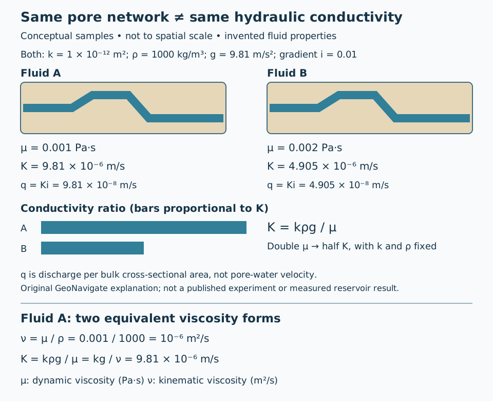
Worked example: change viscosity, hold everything else fixed
Choose hypothetical k = 10⁻¹² m², ρ = 1000 kg/m³ and g = 9.81 m/s². These are illustrative inputs, not measurements or a specified water temperature.
| Quantity | Fluid A | Fluid B |
|---|---|---|
| Dynamic viscosity μ (Pa·s) | 0.001 | 0.002 |
| Hydraulic conductivity K (m/s) | 9.81 × 10⁻⁶ | 4.905 × 10⁻⁶ |
| K (m/day) | 0.847584 | 0.423792 |
| Specific discharge q at i = 0.01 (m/day) | 0.00847584 | 0.00423792 |
For A, substitute 10⁻¹² × 1000 × 9.81 / 0.001. Convert seconds to days by multiplying by 86,400. B's denominator doubles, so its conductivity halves. Applying q = Ki with i defined as the positive head-loss magnitude per flow distance gives the last row. For a hypothetical 2 m² bulk section, Q = qA is 0.01695168 m³/day for fluid A. These calculations do not describe a real well.
How to describe a test result
Record the fluid, temperature, units and test direction alongside a reported conductivity. Temperature changes density and viscosity, so K can change even when pore geometry does not. Do not equate high porosity with high permeability: pore connections matter. In multiphase work, distinguish absolute permeability from relative permeability before applying a single-phase example.
References and provenance
Groundwater Project, Hydrogeologic Properties of Earth Materials and Principles of Groundwater Flow, §4.4 — primary educational source, read 25 October 2026. Original GeoNavigate explanation, hypothetical arithmetic and artwork. Also consult SLB: absolute permeability and USGS: Klamath Basin hydraulic properties for terminology and hydrogeological context.
Continue learning
Compare the Darcy-flow example and aquifer storage guide. Discuss geological support with Chaser Geological services or contact the team.
Porosity: add pore volumes before averaging
Total porosity uses bulk rock volume as its denominator. The Groundwater Project definition therefore leads directly to a volume-weighted result when several disjoint rock volumes are considered together.
Worked example: unequal represented volumes
Suppose region A has bulk volume 100 cm³ and total porosity 10%. Its pore volume is 10 cm³. Region B has bulk volume 300 cm³ and porosity 30%, hence 90 cm³ of pores. Both values use the same measurement convention and sample conditions. Combined pore volume is 100 cm³ and combined bulk volume is 400 cm³, giving 25%.
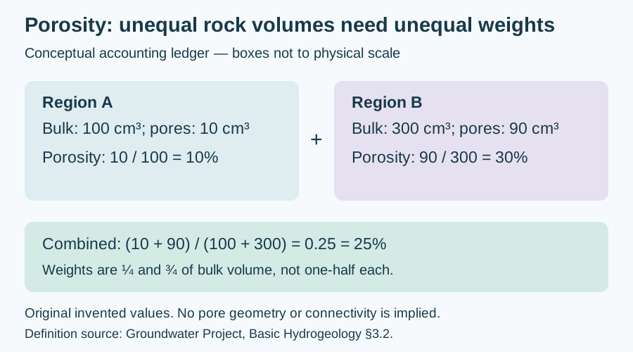
The arithmetic mean, (10% + 30%)/2 = 20%, gives the two regions equal weight even though B represents three times the volume. In general, φ = Σ(φᵢVᵢ)/ΣVᵢ, with φᵢ entered as fractions or consistently as percentages. The volume weights here are 0.25 and 0.75; 0.25×10% + 0.75×30% = 25%.
Apply the right volume boundary
This is accounting over separate, non-overlapping regions; it is not an experiment mixing loose chips into a container. Such a container introduces spaces between chips. For layers covering the same area, bulk volumes are proportional to thickness, so thickness weighting follows. Unequal areas require the actual represented volumes. A deviated borehole's measured interval length is not automatically true bed thickness.
Do not mix total and effective porosity conventions, duplicate overlapping intervals, or silently assign unsampled rock the properties of a convenient plug. This budget establishes neither connected porosity nor permeability. Original hypothetical calculation checked 31 October 2026; no private data or external expert review claimed. Compare the Oilfield Glossary, measurement conventions and Chaser Geological services.
Worked unit check: dynamic versus kinematic viscosity
For fluid A above, kinematic viscosity is ν = μ/ρ = 0.001/1000 = 10⁻⁶ m²/s. Substitute μ = ρν into K = kρg/μ to obtain K = kg/ν. Then K = (10⁻¹² × 9.81)/10⁻⁶ = 9.81 × 10⁻⁶ m/s, exactly the earlier result.
The unit check is (m² × m/s²)/(m²/s) = m/s. Inserting ν into the dynamic-viscosity denominator while retaining ρ is dimensionally wrong; the two viscosity quantities are not interchangeable. Record the quantity and units before conversion. For non-Newtonian drilling fluids, a shear-dependent apparent viscosity requires its measurement conditions and an appropriate flow model.
Concept source: NASA Glenn: Viscosity, read 30 October 2026. Original algebra and hypothetical liquid calculation; NASA's air-property examples are not being used as liquid measurements. Compare the Oilfield Glossary entry.
Worked example: flow along and across layers
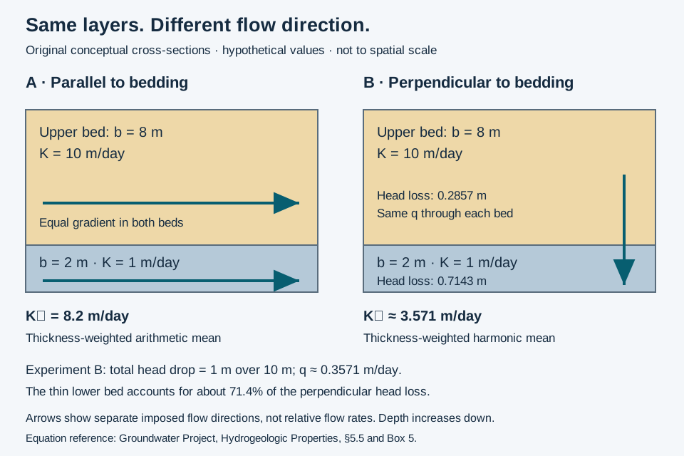
Consider an invented saturated stack: an 8 m layer with K = 10 m/day over a 2 m layer with K = 1 m/day. Both layers are homogeneous, isotropic and laterally continuous. Use steady, single-phase Darcy flow, the same fluid, no internal sources or sinks, and separate experiments with flow strictly parallel or perpendicular to bedding.
Two directions, two averages
Parallel flow shares a head gradient between beds: K∥ = Σ(bᵢKᵢ)/Σbᵢ = (8 × 10 + 2 × 1)/10 = 8.2 m/day. Perpendicular flow must cross both beds at the same specific discharge: K⊥ = Σbᵢ/Σ(bᵢ/Kᵢ) = 10/(8/10 + 2/1) = 3.571 m/day. The ratio K∥/K⊥ is 2.296; state this convention because some software asks for its reciprocal.
Impose a 1 m head drop across the 10 m stack in the perpendicular experiment. The gradient magnitude is 0.1, so q = K⊥i = 0.3571 m/day. Head losses are qb/K: 0.2857 m in the upper bed and 0.7143 m in the lower bed, summing to 1 m. The thinner, less conductive bed takes most of the head loss. Head includes elevation and pressure; downward flow is imposed here, not inferred from gravity alone.
What this example cannot establish
Layered heterogeneity can produce bulk anisotropy. These equivalent conductivities apply to the specified ideal experiments. Discontinuous beds or flow around a partially penetrating well need a more complete model. Bakker's numerical study shows that calibrated effective anisotropy can depend on flow geometry and layer order; it is not a universal aquifer constant.
Sources checked 26 October 2026: Groundwater Project §5.5 and Bakker, The Effective Vertical Anisotropy of Layered Aquifers. Original explanation and arithmetic; no site-specific prediction or expert review is claimed.
Worked comparison: electrical anisotropy is a different property
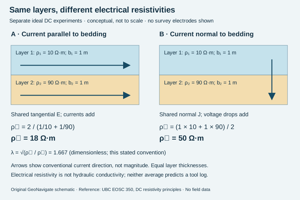
Layering can influence both groundwater flow and electric current, but the property and averaging convention must be named. This invented DC example uses two continuous horizontal beds, each 1 m thick, with isotropic electrical resistivities 10 and 90 Ω·m. Assume linear Ohmic behaviour, steady current, ideal contacts and no internal current sources. Treat parallel and normal current as separate imposed experiments.
Derive the averages from the boundary conditions
Parallel to bedding, tangential electric field E is shared. Current density in each bed is Jᵢ = E/ρᵢ. Averaging J over the equal layer areas gives ρ∥ = 2/(1/10 + 1/90) = 18 Ω·m. This is the harmonic mean of resistivity, equivalently the reciprocal of the arithmetic mean of electrical conductivity.
Normal to bedding, continuity requires the same current density J through both beds. Each voltage drop is Jρᵢbᵢ, so the total divided by total thickness gives ρ⊥ = (1 × 10 + 1 × 90)/2 = 50 Ω·m. This is the arithmetic mean. With the convention λ = √(ρ⊥/ρ∥), λ = 1.667; the resistivity ratio itself is 2.778, not 1.667.
Check the result without a survey interpretation
At imposed parallel E = 1 V/m, the two current densities are 0.1 and 0.011111 A/m². Their equal-area mean is 0.055556 A/m²; E/J gives 18 Ω·m. In a separate normal experiment, impose J = 0.02 A/m²: the bed fields are 0.2 and 1.8 V/m, giving drops of 0.2 and 1.8 V across the 1 m beds. Total field is 2 V/2 m = 1 V/m, yielding 50 Ω·m. These stipulated boundary conditions are not measurements.
Do not insert these resistivities into Darcy’s law. Hydraulic conductivity has different units and fluid dependence. Nor does the sketch predict apparent resistivity from a surface array, induction tool or propagation tool: those require the actual geometry and a forward response. Use electrical anisotropy with explicit axes and scale, and compare its oilfield usage.
Source checked 30 October 2026: UBC EOSC 350, physical principles of DC resistivity, anisotropic ground and charge distribution. Original worked arithmetic and artwork; no private well data or expert review claimed. For applied work, see Chaser Geological services.
Total versus effective porosity: compare like with like
Total porosity counts pore volume relative to bulk volume. Effective porosity requires a convention: core analysis commonly emphasizes connected space, while log interpretation commonly removes clay-bound water. Drying conditions also matter. Do not silently apply both corrections to every reported value.
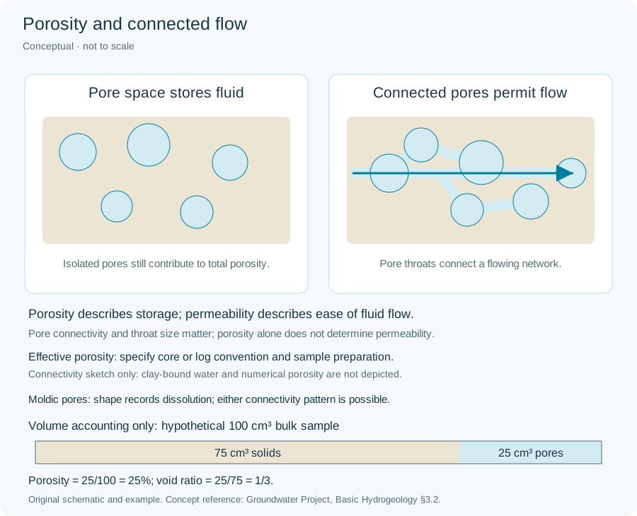
Worked accounting example
Take an invented 100 cm³ bulk sample with 25 cm³ total pore space. Suppose 2 cm³ is isolated and a separate 4 cm³ of the connected space contains clay-bound water. All volumes share the same stipulated reference state; this is bookkeeping, not a laboratory protocol.
- Total porosity: 25/100 = 25%.
- Connected-space convention: (25 − 2)/100 = 23%.
- Total-minus-clay-bound-water convention: (25 − 4)/100 = 21%. In this stipulated case that number still includes the isolated 2 cm³.
- Explicitly excluding both non-overlapping volumes gives (25 − 2 − 4)/100 = 19%. Label this chosen basis rather than presenting it as the universal meaning of effective porosity.
The 23% and 21% results differ by 2 percentage points without requiring a change in the rock. If the two excluded volumes overlap in another model, subtracting both in full would double-count the overlap. If drying changes the sample or its reference volume, the fixed-volume assumptions here no longer hold.
Use the distinction in a well comparison
Before treating a core/log discrepancy as a formation change, compare preparation, measurement method, clay treatment and depth match. Preserve the reported value and its basis alongside any recalculation. None of these four percentages measures permeability or recoverable hydrocarbon volume. A through-going connection in a drawing is also not a flow test.
Concept sources checked 29 October 2026: SLB Energy Glossary, effective porosity (core and log usages) and total porosity. Original hypothetical arithmetic; no well data, reproduced artwork or expert review claimed. Compare the Oilfield Glossary and Chaser Geological services.