
GEONAVIGATE / RESOURCES / SEDIMENTOLOGY
Grain size, sorting and shape: a practical sediment guide
Separate particle size, size spread and grain shape, with phi conversions, compaction balances, facies-migration examples and reliable rock descriptions.
Describing fine-grained rock? Compare fissility, lamination and tectonic cleavage.
Describe four properties independently
A sandstone can be fine grained, well sorted and angular at the same time. These words describe different observations. Grain size describes particle dimensions; sorting describes the spread of sizes; roundness describes edge and corner curvature; and sphericity concerns three-dimensional proportions. Record each before interpreting transport or reservoir quality.
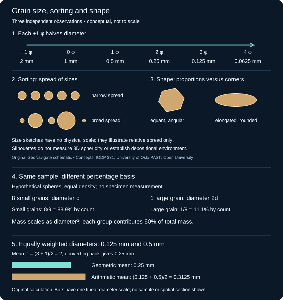
Worked conversion: millimetres to phi
The phi scale makes multiplicative size steps equally spaced. Use φ = −log₂(d / 1 mm), with positive diameter d. The inverse is d = 2−φ mm. A diameter of zero has no finite phi value; do not convert an unmeasured fine fraction to zero diameter.
- A 0.18 mm grain gives −log₂(0.18) = 2.47 φ, rounded. It lies within fine sand on the Wentworth scale.
- A 0.36 mm grain gives 1.47 φ and lies within medium sand. Doubling diameter decreases phi by exactly one.
- A 3.5 φ grain has diameter 2−3.5 = 0.0884 mm, or 88.4 µm: very fine sand.
Sand spans approximately 0.0625–2 mm. Common internal boundaries are 0.125, 0.25, 0.5 and 1 mm. Declare how exact boundary values are assigned instead of hiding rounding differences. Clay-size limits also differ between geological and soil schemes; a size-class name does not identify a clay mineral.
Worked comparison: size spread is not average size
Consider two invented observations: sample A has grains from 0.16 to 0.20 mm; sample B spans 0.08 to 0.80 mm. Their coarse/fine diameter ratios are 1.25 and 10. Their observed phi spans are log₂(1.25) = 0.32 and log₂(10) = 3.32. Sample B has the broader observed spread. These ranges alone do not establish a formal sorting class: neither example specifies the complete distribution or its weighting.
For quantitative work, retain size-fraction weights or counts and report the chosen statistical method. A mass-weighted sieve distribution and a number-weighted image count answer different questions. A few large particles can contribute much of a sample’s mass while representing very few counted grains. Incomplete fine fractions and truncated coarse tails affect calculated parameters.
Roundness and sphericity: avoid the look-alike trap
An equant particle may retain sharp corners. An elongated particle may have smooth ends. Neither silhouette alone establishes a numerical three-dimensional sphericity value. Examine multiple orientations when possible, state the visual comparison method, and keep shape observations separate from mineral identification. Do not infer a unique transport distance from roundness: source texture, mineral durability, recycling and breakage also matter.
A practical wellsite description sequence
- Record sample depth, lag correction, preparation and possible cavings or contamination before assigning the material to an interval.
- Distinguish individual detrital grains from cemented rock chips. Chip diameter is not necessarily original grain size. Use calibrated magnification or a comparator and retain a range as well as the dominant size.
- Describe sorting and shape separately, then record composition, matrix, cement and visible pore character. Do not replace those observations with a depositional-environment label.
- Check whether washing removed fines or drilling created angular fragments. Compare adjacent samples and available core or logs before interpreting a trend.
An example observation might read: “Sandstone, dominantly fine sand; observed grains 0.16–0.20 mm; narrow visual size spread; subangular grains; sphericity not assessed.” It does not establish permeability, depositional energy or a formal statistical sorting class. Cementation, compaction, clay distribution and pore connectivity need separate evidence. See oilfield grain-size terminology and the wellsite manual.
From grain shape to clast fabric
Shape describes an individual particle; fabric describes how particles are arranged. Clast imbrication is an overlapping inclined arrangement. In the upstream-dipping fabric illustrated below, reversing the dip direction gives a candidate paleocurrent direction. A clast’s longest axis is a separate measurement and need not point downstream.
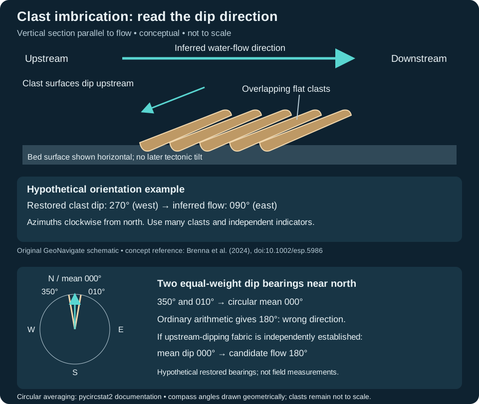
Worked orientation example: assume bedding has been restored to its depositional attitude and several flat clasts share a dip azimuth of 270° (west). For this upstream-dipping fabric, inferred flow is (270° + 180°) modulo 360° = 090° (east). Azimuths are clockwise from north. This calculation reverses a direction; it does not restore tilted bedding.
Collect multiple measurements, document the measured surface and check independent sedimentary indicators. Mixed populations should be kept separate. The Huangshui Valley study by Miao et al. (2008) illustrates the value of systematic clast observations for reconstructing former drainage. Loose drill cuttings have lost their original spatial orientation; do not turn a chip’s apparent inclination into a compass direction. These added sources were checked 25 October 2026.
References and scope
Original GeoNavigate teaching examples, calculations and artwork. No well dataset or third-party figure is reproduced. Sources checked 24 October 2026:
- IODP Expedition 331, Methods, Table T1: millimetre, phi and Wentworth comparisons.
- University of Oslo Natural History Museum, PAST grain-size analysis: distribution inputs and statistical methods. Its prose sand-diameter inequality is reversed; the numeric bounds are checked against the IODP table.
- Open University, The geological sorting hat: sorting, roundness and grain form.
- Ocean Drilling Program sedimentary-rock laboratory: independent textural observations.
Browse the Geology Dictionary, explore Chaser Geological wellsite services, or contact Chaser Geological.
Worked example: a cut face can miss a clast contact
Clast-supported texture concerns a touching framework, as described in the IODP Expedition 350 methods. A cut surface is only one intersection through that three-dimensional arrangement. A gap on that surface need not mean the neighbouring clasts are separated everywhere.
Consider two ideal spheres, both radius R = 5 mm, with centres at (0, 0, 0) and (10, 0, 0) mm. Their centre spacing is 10 mm, exactly twice their radius, so they touch at (5, 0, 0). This is an invented geometric example, not a rock reconstruction. The z coordinate is perpendicular to the section planes; it is not geological depth.
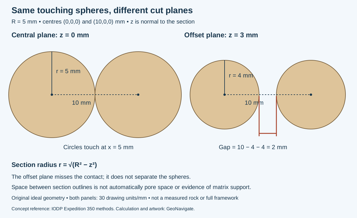
Calculate the offset section
A plane z = h cuts a sphere into a circle whose radius is r = √(R² − h²), for |h| ≤ R. This follows from the right triangle between the sphere centre, section-circle centre and a point on its rim.
- At h = 0, r = 5 mm. The two circles meet because their radii sum along the centre line to 10 mm.
- At h = 3 mm, r = √(25 − 9) = 4 mm.
- The section-circle centres remain 10 mm apart. The visible gap is 10 − 4 − 4 = 2 mm.
The contact at z = 0 still exists; the offset plane simply misses it. The gap represents space between the sphere intersections on that plane, not a measured pore aperture. In a real specimen that space could contain finer material, cement or pores, which must be described independently.
Use the geometry without overinterpreting it
One touching pair does not establish a load-bearing or specimen-wide framework. Conversely, a few apparently isolated clasts in one image do not establish matrix support throughout the specimen. Inspect representative surfaces, note the observation plane, and keep contact evidence separate from clast abundance, roundness and inferred depositional process. Loose cuttings have lost their original arrangement and cannot reconstruct it merely by being placed next to one another.
Source terminology checked 31 October 2026; original derivation and artwork. No private samples or reproduced publication figures. See Oilfield Glossary, Chaser Geological services or contact Chaser.
Worked example: a circular view can hide flattening
Sphericity describes three-dimensional form. A silhouette records only one projection. This ideal-shape exercise shows the missing information without assigning a numerical sphericity score.
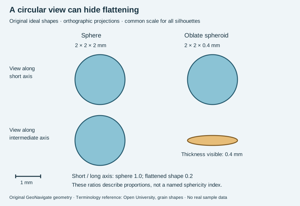
Compare two known three-dimensional objects
Shape A is a sphere with diameter 2 mm. Shape B is an oblate spheroid with full orthogonal dimensions 2 mm, 2 mm and 0.4 mm. Looking along the shortest axis, both project to a circle of diameter 2 mm. A top-view photograph alone cannot distinguish them under this ideal geometry.
Turn the objects to view along an intermediate axis. Shape A remains circular; B projects to an ellipse 2 mm wide and 0.4 mm high. Their short-to-long axis ratios are 2/2 = 1 and 0.4/2 = 0.2. That calculation describes flattening; it is not automatically the value of a particular published sphericity index. The two equal longest axes of B make the chosen in-plane viewing direction immaterial here.
Apply the lesson to a rock description
For loose grains, document more than one orientation and state whether dimensions are measured or estimated. A photograph of chips lying flat can hide thickness. A thin section introduces a different issue: it cuts through grains instead of showing their full projected outlines. Preserve that distinction in the observation record.
Describe corner and edge roundness separately. The smooth ideal surfaces here do not demonstrate any particular abrasion history, transport distance or depositional environment. Do not treat multi-grain cuttings as single sediment grains without checking their texture. Compare the Oilfield Glossary entry.
Terminology reference checked 31 October 2026: Open University, The geological sorting hat, grain-shape comparison. Geometry and example are original; no source figure reproduced. Chaser Geological services.
Worked example: average phi or average diameter?
Give two hypothetical diameter observations, 0.125 and 0.5 mm, equal weight. Their phi values are 3 and 1; mean phi is 2, which converts to 2⁻² = 0.25 mm. This equals their geometric mean, √(0.125 × 0.5). Their arithmetic diameter mean is instead 0.3125 mm. The lower bars in the shared diagram show this 1.25:1 difference.
The inputs did not change; the averaging operation did. Report the variable, weighting and method before interpreting a difference between sample reports. This two-observation exercise is not a full sieve analysis or a Folk–Ward graphical mean. Compare phi scale and sorting. Method context: University of Oslo PAST grain-size documentation; conversion values: IODP 331 Table T1. Original invented calculation.
Worked example: grain counts are not mass fractions
A photographed grain population and a weighed sieve fraction describe different distributions. The University of Oslo PAST documentation expects weights or weight percentages for sieve fractions. Do not substitute image counts into that input without a justified conversion. Sorting still concerns the spread of sizes; a method and weighting are needed for a numerical result.
Imagine eight spherical grains of diameter 0.25 mm and one spherical grain of diameter 0.50 mm, all with identical density. This is invented arithmetic, not a measured sediment sample. Sphere volume is πd³/6, so doubling diameter gives eight times the volume and mass. The eight small grains together therefore weigh the same as the one large grain.
- By number: small grains are 8/9 = 88.9%; the large grain is 1/9 = 11.1%.
- By mass: the small-grain group contributes 8 relative mass units and the large grain contributes 8, giving 50% each.
- By summed projected area: non-overlapping circular projections would give 8 versus 4 relative area units, or 66.7% versus 33.3%. This is a third basis, not either of the first two.
The shared full-size sediment-texture schematic includes this count/mass comparison. The example does not assign a formal sorting class, establish mineral proportions or predict permeability.
Apply the distinction to wellsite images
Record whether the counted objects are individual liberated grains or multi-grain rock chips. State the sample interval, preparation, image scale, selection rule and minimum resolvable size. Overlap, broken particles and excluded fine material can change the visible population. A washed-cuttings photograph does not by itself establish the complete formation grain-size distribution.
Do not apply the sphere conversion to irregular mixed-mineral chips as though their three-dimensional volumes and densities were known. Preserve the raw observations and compare equivalent populations before reporting a trend. See density, oilfield sorting terminology and Chaser wellsite services. Original explanation and calculations checked 29 October 2026; terminology also checked against SLB sorting. No private samples or external expert review claimed.
Stylolite or open fracture: describe the evidence separately
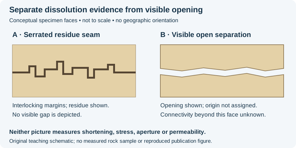
A stylolite is a serrated dissolution surface, commonly highlighted by less-soluble residue. SLB describes interlocking surfaces in carbonate and quartz-rich rocks, with residues such as clay and iron oxides. This is evidence of pressure solution; a dark line by itself is not a diagnostic identification.
Worked description exercise
For invented specimen A, write: “Dark serrated seam with interlocking margins; no visible gap at this observation scale.” Interpret a stylolitic dissolution seam only after checking the contacts and residue. For invented specimen B, write: “Visible separation between matching rock margins.” Record that opening separately from any proposed dissolution history. An opening could overprint an older seam; the two observations are not mutually exclusive.
Keep the inference within the evidence
Do not turn the cartoon tooth height into metres of shortening or a current stress value. There is no calibrated scale or restoration here. Likewise, the open gap in B does not establish a connected flow route through the rock volume. Permeability requires evidence beyond one exposed face, and a cuttings fragment can lose the orientation and continuity visible in intact material.
As a separate invented count, 6 of 15 inspected fragments contain a candidate serrated seam: 40% of those selected fragments. This is neither 40% dissolved rock nor a formation-wide seam abundance. Keep fragment selection, observation scale and identification uncertainty in the record.
Original exercise prepared 28 October 2026; no field data or external expert review claimed. Compare the compaction and cement volume balance and Oilfield Glossary entry. For geological support, visit Chaser services or contact GeoNavigate.
Worked core example: grading within one bed
Graded bedding concerns grain-size change through one bed. Normal grading fines upward; inverse grading, also called reverse grading, coarsens upward. These descriptions follow the sedimentary-structure terminology in IODP Expedition 400 Methods (checked 25 October 2026).
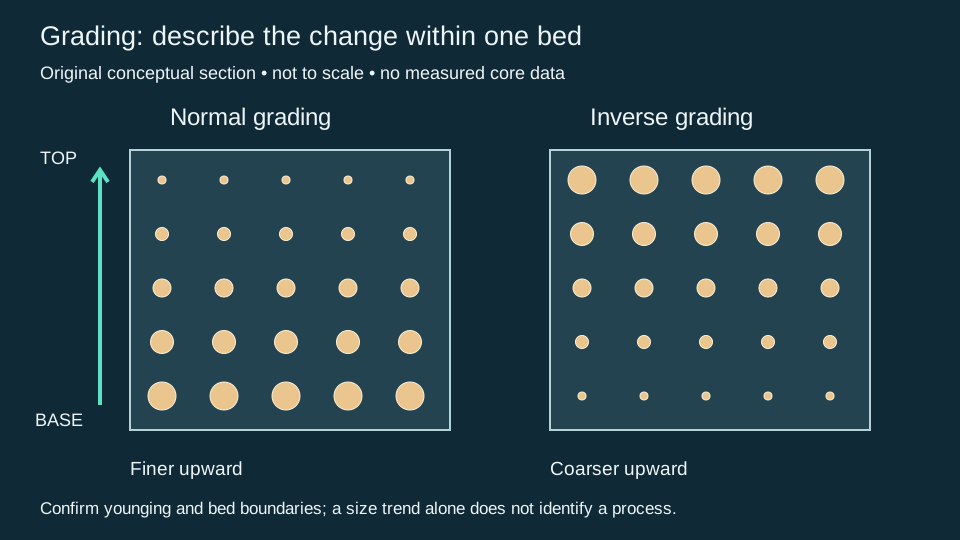
Consider an invented intact, upright 20 cm bed. Comparable samples at 2, 10 and 18 cm above its base have measured median grain diameters of 0.50, 0.25 and 0.125 mm. The median diameter decreases upward by a factor of four, corresponding to 1, 2 and 3 phi. These observations support normal grading over the sampled interval; three measurements do not demonstrate a smooth trend at every intervening level.
Reversing those diameters gives an inverse trend. Combining samples from several beds, however, would answer a different question about a bedset or succession. Record the sampled interval, grain population and measurement method before comparing trends. A log response is not a direct grain-size measurement.
Keep the observation and interpretation traceable
- Identify the bed boundaries and document core orientation, recovery gaps and disturbance. Establish stratigraphic younging independently where overturning is possible.
- Measure equivalent grain populations at several levels. Distinguish the size of a rock chip from the grains within it, and dominant grain size from isolated outsized clasts.
- Record the observed pattern before assigning a process. Compare contacts, lamination, fossils and surrounding facies. Neither normal nor inverse grading uniquely identifies a depositional environment.
Loose cuttings can mix material over depth and lose bed-scale fabric; qualify any inferred grading accordingly. A turbidite interpretation needs context beyond a fining trend. Compare the oilfield grading entry and the wellsite description workflow. This is an original teaching example, with no measured well data or claimed expert review.
Flute and groove casts: distinguish a direction from an axis
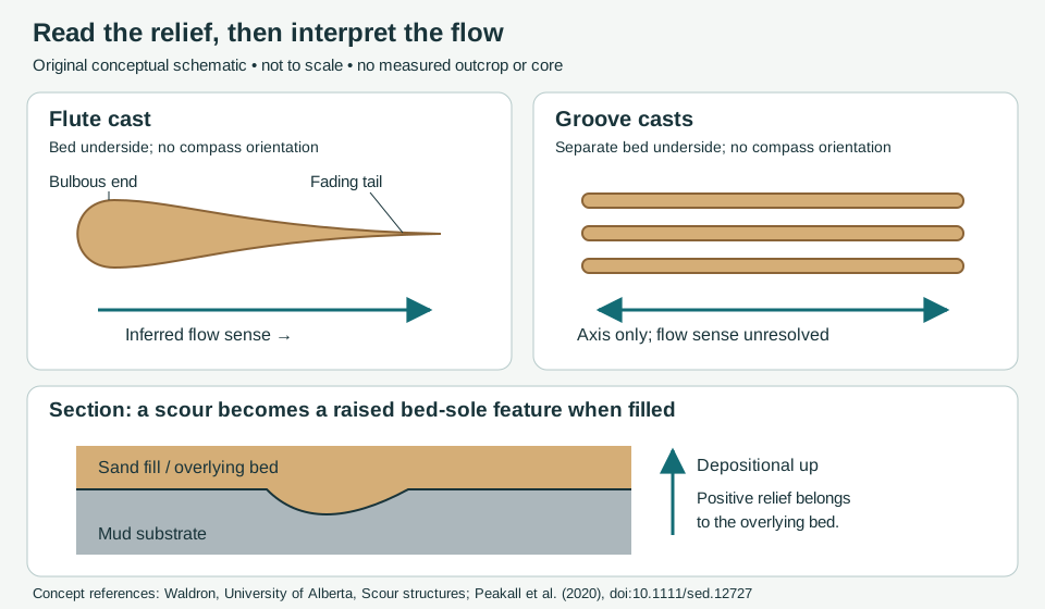
Inspect bed undersides as well as grain texture. A flute cast preserves the fill of a scoop-shaped scour. A groove cast preserves the track of a dragged object. Both are examples of sole markings. Record the relief and its relation to the overlying bed before drawing a flow arrow.
Worked example: the 035°/215° ambiguity
Suppose an oriented, horizontal bed sole carries straight uniform groove ridges aligned 035°–215°. Bearings are clockwise from true north. The opposite bearing is (035° + 180°) modulo 360° = 215°. Report the axis as 035°/215°, with flow sense unresolved. Averaging those two equivalent axis bearings arithmetically gives 125°, which points across the grooves and is not a valid flow estimate.
In a separate hypothetical exposure, a well-preserved flute has its bulbous end toward 215° and its fading tail toward 035°. Its morphology supports flow toward 035°. Do not transfer this sense to the first exposure without evidence that the records are comparable. Nor should arrows be added to every groove simply because a nearby bed has a directional indicator.
A traceable observation workflow
- Record bed identity, stratigraphic younging, viewing face, north reference, bedding attitude and whether the sample retains geographic orientation. The section above uses depositional up; an overturned outcrop needs separate orientation work.
- Describe a positive ridge or bulb on the bed base separately from a negative scour in the underlying surface. Photograph with a scale and orientation marker; retain uncertain identifications.
- Record several structures, their spread and any cross-cutting relationships. For tilted beds, restore orientations with a documented structural method before comparing paleoflow bearings. Adding 180° reverses a bearing; it does not undo bedding tilt.
- Keep an observed axis, a morphology-based flow sense and an environmental interpretation in separate fields. Unoriented drill cuttings cannot supply a geographic bearing. For core, document both recovery and orientation control.
The process review by Peakall and colleagues shows why a simple “sole mark equals turbidity current” rule is inadequate: different flow types can make these structures, and erosion may precede the flow that deposits the overlying sand. Use contacts, internal structures and surrounding facies alongside sole markings. Do not infer velocity or a unique depositional environment from the two teaching shapes alone.
Compare paleocurrent, turbidite, the oilfield flute-cast entry and the clast-fabric example. Sources checked 26 October 2026. This is an original teaching exercise, without private well data or a claimed expert review. For geological support, contact Chaser Geological.
Worked core example: describe a deformed bed contact
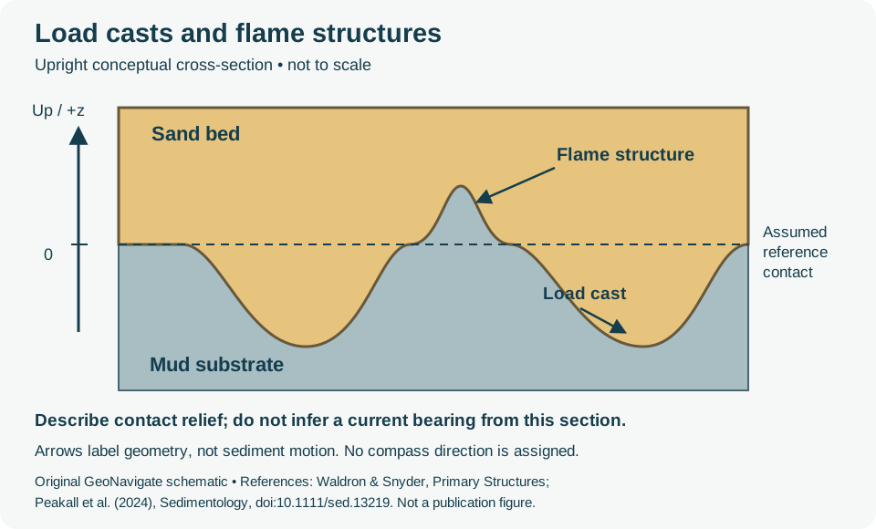
A load cast is a downward bed-base bulge; a flame structure is an upward mud tongue between such bulges. These are soft-sediment deformation features. Compare their geometry with the scour-and-fill structures above before assigning a process.
Separate the observation from the reconstruction
Consider an invented intact, upright core slab. For this exercise only, assume a formerly flat contact and set it to z = 0 mm, with z positive upward. The deepest sand lobe reaches z = −30 mm and the highest mud tongue reaches z = +20 mm. The observed vertical envelope is therefore 20 − (−30) = 50 mm. This describes the extremes in this section. It is neither a settlement measurement nor a strain, velocity or deformation-rate calculation.
In real core, the original contact may be unknown. State the chosen reference and report visible relief rather than silently treating a reconstructed surface as measured. Keep core depth, which commonly increases downward, separate from this local positive-up coordinate. Do not combine measurements from differently oriented slabs without documenting the transformation.
What to record before interpreting
- Record lithology on each side, contact shape, preserved lamination, scale, recovery gaps and any drilling disturbance. Photograph the slab with an orientation mark.
- Describe whether the feature is isolated or repeated and whether a plan view is available. A single section cannot fully describe three-dimensional form.
- Keep an observed inclination separate from an inferred current direction. The review by Peakall and colleagues discusses several causes of inclined loads, including slope and unequal loading, as well as flow effects.
- Use surrounding beds and independent way-up evidence to assess orientation. Do not diagnose an earthquake trigger from the presence of a load or flame alone; this example contains no trigger evidence.
For wellsite reporting, use the Oilfield Glossary load-cast entry and sample-description workflow. Loose cuttings cannot retain the intact contact shown here. Contact Chaser Geological for service enquiries.
Sources and scope
Sources checked 26 October 2026. Original teaching example and artwork; no expert review claimed.
- Waldron and Snyder, Geological Structures: a Practical Introduction — Primary Structures: load and flame terminology.
- Peakall et al. (2024), Flow-induced interfacial deformation structures, Sedimentology, DOI 10.1111/sed.13219: section “Differentiating FIDS from load casts and flames.” Not every bed-sole ridge is an erosional groove; record geometry and internal structure before classification.
Worked core example: folded laminae and deformation extent
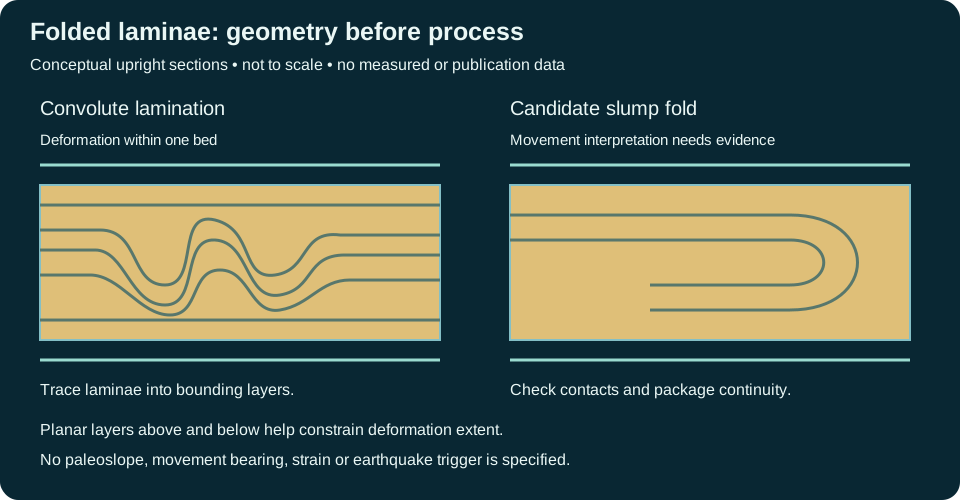
Convolute lamination describes folded laminae within a bounded bed. A slump fold includes a process interpretation: downslope movement while sediment was soft. Keep the observed geometry and the evidence for movement in separate parts of the description.
Describe an interval before assigning a cause
In an invented complete, upright core interval, the bed extends from 1250.10 to 1250.40 m measured depth. Folded laminae occur between 1250.16 and 1250.34 m. The bed occupies 0.30 m along core, and visible deformation spans 0.18 m, or 60% of that recovered bed interval. This fraction describes along-core extent. It is not shortening, strain, settlement or the fraction of the sediment volume that moved. Core length is not true stratigraphic thickness unless borehole and bedding geometry justify that conversion.
A suitable observation is: “Contorted laminae in the central 0.18 m of a 0.30 m recovered bed; laminae become planar toward the contacts; adjacent beds remain planar in this slab.” Convolute lamination is a defensible descriptive label. A slump interpretation additionally needs evidence for soft-sediment displacement, such as a consistent package geometry and associated slide surfaces or disrupted beds. A single narrow core may not resolve those relationships.
- Record core depth convention, recovery, breaks, orientation and possible coring disturbance. Do not bridge missing core as though continuous laminae were observed.
- Trace laminae to bed boundaries. Compare bed-confined deformation with deformation extending across several beds and with later tectonic fabrics.
- Describe loads, mud flames and possible water-escape features independently. Association supports a process discussion but does not uniquely establish a trigger.
- Use lateral exposure, multiple cores or independent structural evidence before inferring paleoslope or movement direction. Fold asymmetry alone does not demonstrate an earthquake or a compass bearing.
Loose cuttings generally lose these relationships. Use the oilfield definition and wellsite description workflow for reporting limitations. Contact Chaser Geological for service enquiries.
Sources and scope
Checked 26 October 2026: IODP Expedition 397 Methods, section 2.7 supplies the classification context; University of Alberta, soft-sediment deformation and dewatering illustrates associated structures. Original teaching example and artwork; no expert review claimed.
Worked core example: dish laminae and a pillar
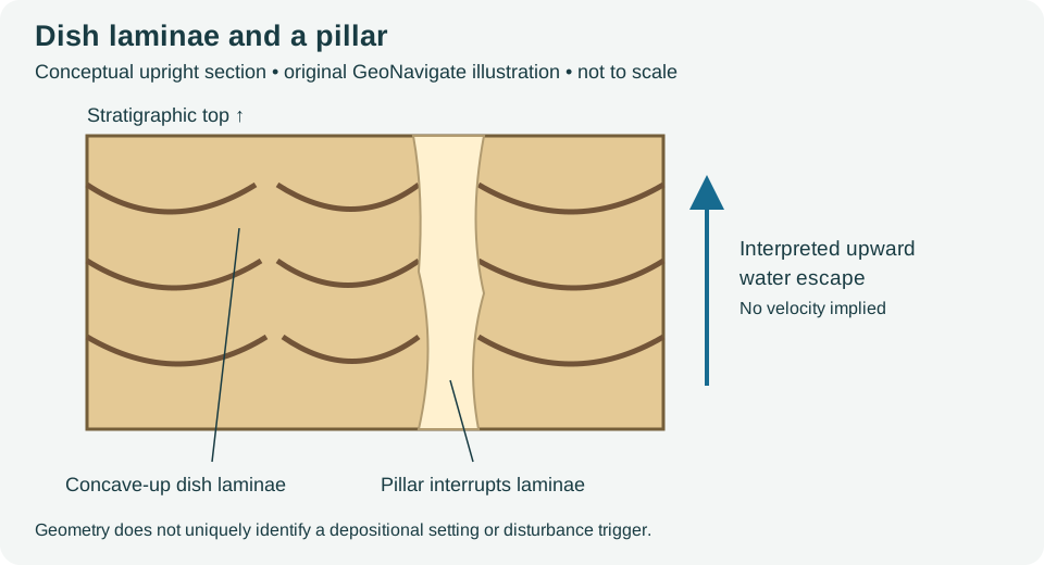
Dish structures and pillars record sediment modification during water escape. Describe the laminae and their interruptions before interpreting the process. Dishes alone do not establish a turbidite, an earthquake trigger or a paleoflow direction.
Measure the feature that is actually visible
In an invented slab, a pale band is 6 mm wide along a horizontal 120 mm traverse. It occupies 6 / 120 × 100 = 5% of that traverse. At a second height, its apparent width is 9 mm, or 7.5%. Report both measurements and their positions. Neither fraction measures porosity, permeability, water loss or the three-dimensional volume occupied by pillars. An oblique cut and an irregular band can change apparent width.
A traceable observation is: “Repeated concave-up dark laminae terminate against a pale, steep band; apparent band width is 6–9 mm at two marked traverses.” A water-escape interpretation should be supported by sediment texture and the surrounding bed relationships. Compare possible burrows, fracture fills and coring damage rather than identifying every pale band as a pillar.
- Record scale, slab orientation, bed contacts, recovery and any disturbance. Establish stratigraphic top independently where overturning is possible.
- Trace dark laminae and the pale band across the available face. A two-dimensional section cannot determine whether the band is a pipe or a sheet.
- Compare nearby convolute lamination and primary structures. Preserve observations that disagree with the interpretation.
- Keep fluid-escape interpretation separate from reservoir-quality predictions. Later cementation and compaction require independent assessment.
Loose cuttings cannot retain the complete geometry. See the oilfield entry, wellsite description workflow and Chaser Geological services.
References and scope
Sources checked 27 October 2026: Lowe and LoPiccolo (1974), linked above, and University of Alberta, soft-sediment deformation and dewatering structures. Original hypothetical measurement exercise; no private well data, third-party photograph or expert-review claim.
Worked ripple example: an axis is not a flow direction
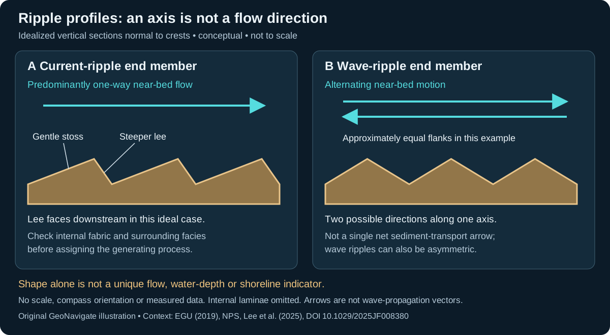
Current ripples and wave ripples record motion over a sediment bed. Describe the preserved geometry first. In the ideal current example below, the gentler stoss flank rises toward the crest and the steeper lee flank faces downstream. The wave example shows an oscillatory end member, not a rule that every wave ripple must be symmetric.
Hypothetical horizontal bed: keep two observations separate
| Observation | Geometric result | Interpretation limit |
|---|---|---|
| Approximately straight crests trend 030°–210°; a profile is measured normal to them. | The normal axis is 120°–300°. | An axis has two ends, not one directed paleocurrent. |
| In that profile the shorter, steeper flank faces 120°. | If independently identified as a migrating current ripple, the downstream interpretation is toward 120°. | The shape alone does not exclude wave asymmetry or combined flow. |
| The two flanks are approximately equal instead. | Record approximate symmetry and the same 120°–300° axis. | Do not assign net transport toward either end from this observation alone. |
The arithmetic is simply 030° + 90° = 120°; the opposite heading is 300°. This is a horizontal-bed teaching case. A tilted bed needs an appropriate structural restoration before a geographical paleoflow interpretation. An oblique cut can misrepresent the profile, and an unoriented slab cannot provide these compass headings.
Use context to test the process
Inspect crest continuity, multiple profiles, lamination, contacts and nearby cross-bedding. Document whether a surface is an original bed top or a cast before using it as a younging indicator. A ripple shape is not a unique water-depth, shoreline or velocity measurement.
Lee and colleagues tested waves, currents and combined flow over a sloping sand bed and found that geometry depends on both the flow combination and local slope. That is a reason to retain competing interpretations, not a formula for extracting an ancient current speed from this sketch. At the wellsite, record the intact fabric and orientation evidence; loose cuttings usually cannot retain the crest-to-profile relationship.
References checked 27 October 2026: NPS, Ancient Ripple Marks; Papeschi, EGU (2019); and Lee et al. (2025), Observation and Prediction of Sand Ripple Geometry on a Sloped Bed Under Varying Combined Wave-Current Flows (institutional abstract read). These original examples and drawings are not publication figures or measured results. Compare oilfield terminology, the wellsite workflow, or contact Chaser Geological.
Worked core description: what forms the framework?
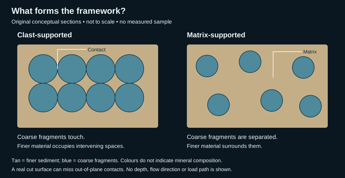
Clast-supported texture and matrix-supported texture separate two contact arrangements. IODP Expedition 350 uses the first for a coarse framework and the second for larger fragments enveloped by smaller particles. Its matrix can itself contain particles larger than sand; the word does not mean clay alone. Use a stated descriptive scheme, rather than an unexplained percentage cutoff.
Three hypothetical observations
| Sample | Observation | Defensible record |
|---|---|---|
| A: intact gravel bed | Rounded fragments touch across several exposed faces; sand occupies intervening spaces. | Clast-supported conglomerate with sandy matrix. Describe rounding and sorting separately. |
| B: intact gravel bed | Separated rounded fragments are surrounded by finer sediment on the inspected faces. | Matrix-supported conglomerate on the available evidence; document the scale and inspected area. |
| C: washed cuttings | Loose rock chips and fine grains have been separated and mixed during recovery. | Support fabric unresolved. A tray arrangement cannot recreate the original framework. |
Make the interpretation testable
For sample A, sketch several contacts and mark where the surface ends. For sample B, record any local touching clusters instead of concealing them in a single label. If the exposure is too small to decide, retain “support uncertain” and request a larger intact surface or additional section. These are observation checks for this exercise, not a statistical sampling standard.
Keep the support description distinct from breccia versus conglomerate, which describes angular versus rounded coarse fragments. Identify matrix separately from pore-filling cement where possible. Neither panel supplies a permeability measurement or a flow-process diagnosis. Test a proposed depositional interpretation against bedding, grading, contacts, composition and the surrounding succession.
IODP also documents coring-induced remoulding and introduced material; check recovery disturbance before treating the preserved arrangement as depositional. References checked 27 October 2026: Tamura and colleagues (2015), Expedition 350 methods; University of Auckland, Conglomerate. No source artwork is reproduced. Compare the oilfield entry, wellsite geology workflow, or contact Chaser Geological.
Flaser and lenticular bedding: describe continuity before process
Alternating sand and mud can preserve quite different arrangements. In flaser bedding, discontinuous mud streaks interrupt rippled sand, particularly in troughs. In lenticular bedding, sand forms lenses within a muddy background. Lenses can be separate or locally connected. Wavy bedding describes an intervening arrangement with more continuous undulating sand and mud layers; these are descriptive patterns, not a compulsory vertical sequence.
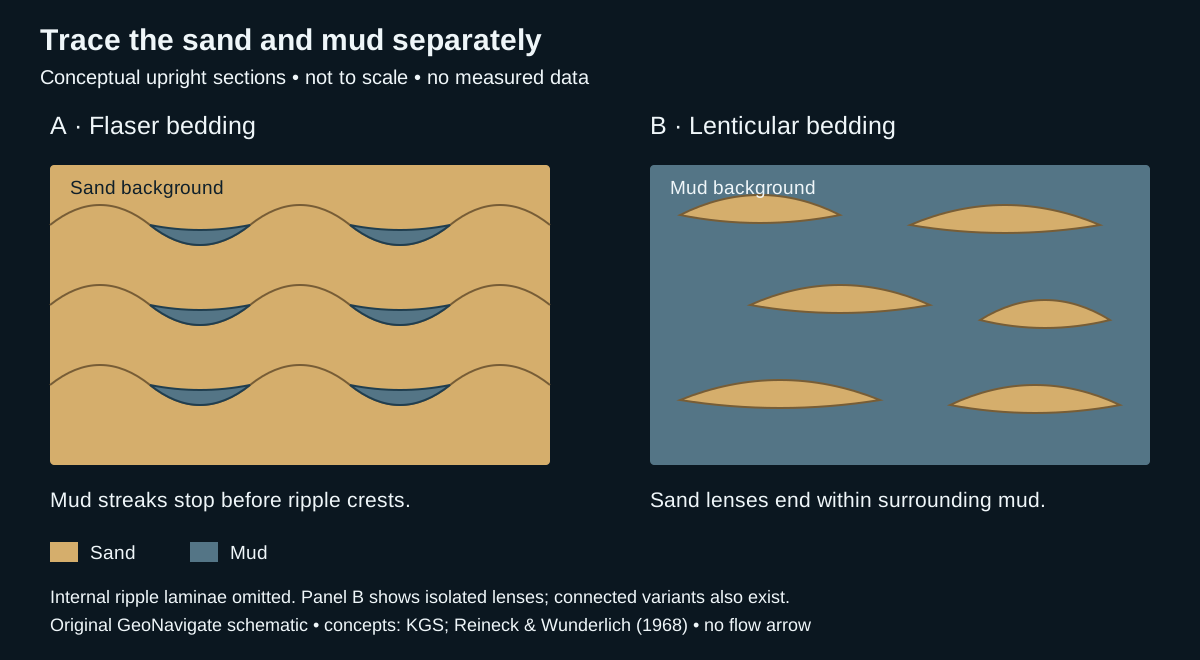
Worked example: two invented intact core faces
Assume upright, undisturbed material with reliable grain-size identification. The following observations are teaching examples, not well measurements. They deliberately omit a sand-percentage cutoff: material proportion alone does not specify the geometry.
- Face A: sand is continuous across the exposed face. Thin muddy streaks occupy several ripple troughs, but vanish toward adjacent crests. Describe flaser bedding, then record streak lengths, thicknesses and whether any mud layer crosses a crest. Do not describe the mud as a continuous seal.
- Face B: mud is continuous around several sand lenses. Most lenses end visibly within the face; two touch locally. Describe lenticular bedding with isolated and locally connected lenses, then record the observed connections. A contact in one slice does not prove connection between wells.
- A bag of chips from either interval: both sand and mud fragments occur, but their original arrangement is lost. Report mixed lithologies with the sampling limitations. The chip mixture alone cannot distinguish A from B.
What additional evidence supports a tidal interpretation?
Alternation between bedload transport and quieter suspension settling can produce these contrasting layers. Tidal settings commonly preserve such alternations, but the bedding names alone do not demonstrate tides. Look for a consistent association of structures, such as mud drapes, changing palaeoflow directions and organized bundles, and assess the surrounding facies. The Kansas Geological Survey Waverly study combines bedding with other observations to interpret tidal-flat environments; its interpretation should not be transferred automatically to an unrelated core.
A repeatable description workflow
- Document recovery, orientation, disturbance and the size of the observed face. Distinguish a depositional lens from deformation, a burrow fill or a broken fragment.
- Identify sand and mud separately. Trace their boundaries across the available exposure and note where visibility ends. Describe internal lamination if preserved.
- Record thickness ranges, local connections and changes between adjacent intervals. A lens-shaped channel body is a different scale of observation from lenticular bedding.
- Keep the description, process interpretation and reservoir hypothesis separate. Permeability, cementation and three-dimensional continuity require their own evidence; a two-dimensional sand connection is not a flow test.
Compare current ripples, facies and the separate Oilfield Glossary. This section extends the texture guide from individual grains to the arrangement of contrasting sediment fractions.
References and scope
- Enos, Jefferson and Goetz (2008), Kansas Geological Survey, Lawrence Formation results — bedding geometry, terminology and limits on a uniquely tidal interpretation.
- Kansas Geological Survey Bulletin 245, Waverly sedimentology — described heterolithic facies and their contextual interpretations.
- Reineck and Wunderlich (1968), Classification and origin of flaser and lenticular bedding, DOI 10.1111/j.1365-3091.1968.tb00843.x — publisher summary and classification checked; no full-paper review claimed.
Original explanation and examples; checked 27 October 2026. No expert review claimed. Browse geology guides, Chaser Geological services or contact GeoNavigate.
Compaction and cement: the same porosity can hide different histories
Before interpreting a tight sandstone, separate framework shortening from filling the space between grains. Mechanical compaction changes packing or grain shape. Pressure solution removes material from stressed contacts and allows shortening. Cement occupies pore space; these processes can interact during diagenesis.
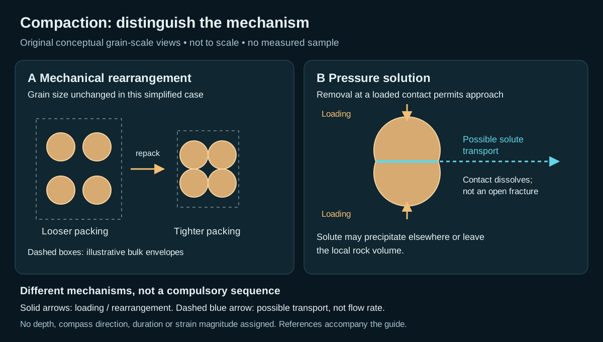
Worked volume balance: state what is conserved
Take an invented, initially uncemented sample with bulk volume 100 cm³, grain volume 60 cm³ and pore volume 40 cm³. Its total porosity is 40/100 = 40%. The following are alternative thought experiments, not successive stages or measured reservoir predictions.
- Mechanical volume reduction: keep grain volume at 60 cm³ and reduce bulk volume to 80 cm³ by rearrangement. Pore volume becomes 20 cm³, so porosity is 20/80 = 25%. Pore volume halves, but porosity falls by 15 percentage points, not 20. The denominator also changed.
- Cement only: retain the initial 100 cm³ bulk volume and add 15 cm³ of cement in the pores. Total solid volume becomes 75 cm³ and pore volume 25 cm³. Porosity is again 25%, although the framework has not shortened in this stipulated example.
The two final porosities are equal. Neither that equality nor a porosity log uniquely separates the histories. Both calculations omit fractures, microporosity, grain compressibility and subsequent dissolution. These assumptions make the arithmetic transparent; they are not a sandstone compaction law or a conversion from porosity to permeability.
Why pressure solution needs another balance
Do not apply the constant-grain-volume assumption automatically to pressure solution. If material dissolves from contacts, identify the chosen system boundary. Material precipitated inside the same boundary can preserve total solid inventory while moving it; exported solute changes that inventory. The local dissolved volume, cement volume and bulk shortening need separate constraints. A stylolite may record localized dissolution, but its visible relief alone is not a complete restoration of missing rock.
What to record at the wellsite and microscope
- Distinguish tight grain packing, deformed or fractured grains, contact truncation and pore-filling cement. Record observations separately from the inferred process.
- Check grain and cement mineralogy and cross-cutting relations across representative material. A few loose cuttings cannot preserve every original contact or establish the history of a whole interval.
- Compare core, petrography and available log evidence. Report unresolved alternatives; do not infer a unique burial depth, pressure or permeability from the cartoon or the volume exercise.
Sources and scope
Concept references checked 27 October 2026: Grier and Marschall, AAPG Reservoir quality; University of Alberta, Planet Earth: sediment and sedimentary rock; Houseknecht (1987), relative importance of compaction and cementation (publisher-indexed abstract; full article not reviewed). Original GeoNavigate arithmetic and illustration, no copied figures, private well data or claimed external expert review. Continue with the Oilfield Glossary, Geology Guides, Chaser Geological services or contact Chaser Geological.
Walther’s law: test a facies interpretation against its neighbours
A facies association groups facies using evidence for a shared depositional context. State the observations and grouping criteria before naming that context. Walther’s law provides a consistency test: where deposition is conformable, neighbouring environments can leave neighbouring facies in a vertical succession as their positions change. It supplies neither a unique environment nor an age correlation by itself.
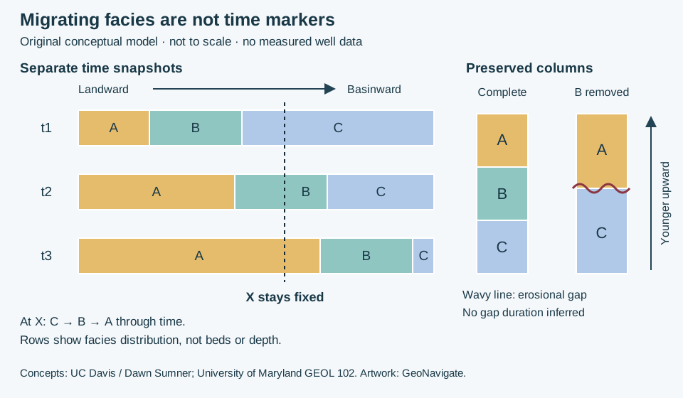
Worked interpretation: follow one location through three snapshots
In this invented model, A, B and C are adjacent facies belts ordered from landward to basinward. Their boundaries move basinward by the same arbitrary distance between each snapshot. Position X remains fixed. At t1, X is in C; at t2 it is in B; at t3 it is in A. With continuous accumulation and preservation at X, the resulting column reads C → B → A from oldest to youngest. Equal snapshot spacing in the drawing does not specify equal sediment thickness, equal time intervals or a migration speed.
For a possible deltaic interpretation, C could represent prodelta mud, B delta-front deposits and A delta-plain deposits. That interpretation needs supporting structures, fossils and geometries; letters and colours alone contain no such evidence. Progradation describes the basinward advance. It does not, by itself, prove a fall in relative sea level. A particular environmental belt can contain several descriptive facies.
Change one assumption: remove the intermediate record
Now suppose erosion removes the B interval before A accumulates. The second column preserves C directly beneath A across the wavy erosional surface. Those two environments need not have been immediate neighbours. The missing B interval has no measurable preserved thickness here; the sketch does not determine how long the gap lasted. Nondeposition could also produce an incomplete record, but that is not the specific removal history drawn.
If a real section appears to skip an expected environment, compare three explanations: incomplete preservation, an unrecognized intervening facies, or an incorrect environmental interpretation. Return to the observed contacts and structures to test them. Do not invent an interval merely to make a preferred facies model fit. In deformed or poorly recovered sections, establish structural order and recovery before treating the apparent stack as a depositional sequence.
Apply the distinction to well correlation
First preserve the sample and log depth references, contact observations and recovery limits. Then compare facies packages between wells. Similar sandstone or gamma-ray character is a correlation hypothesis, not proof of equal age. A migrating facies boundary may be diachronous; seek independent time constraints where available. This model predicts no gamma-ray amplitude, reservoir connectivity, pore pressure or drilling margin.
Sources and scope
- Dawn Sumner, UC Davis: Sediments and Strata — conformability and the distinction between lithological and time correlation.
- Dawn Sumner, UC Davis: Sedimentary Facies — observations, facies and environmental interpretation.
- Dawn Sumner, UC Davis: Interpreting Stratigraphic Columns — testing missing environments against observations.
- University of Maryland GEOL 102: Fluvial and Deltaic Environments — migration and deltaic stacking.
Primary teaching sources checked 27 October 2026. Original explanation and artwork; no publication figure, measured well record or external expert review is claimed. See the Oilfield Glossary, Geology Guides, Chaser Geological services or contact Chaser Geological.
Parasequences: distinguish a flooding contact from maximum flooding
A parasequence is a package bounded by flooding surfaces, not a prescribed number of metres. In shallow-marine interpretation, test the relationship between its facies and the contacts above and below. A marine flooding surface records a deepening interpretation; maximum flooding adds a larger-scale stratigraphic designation.
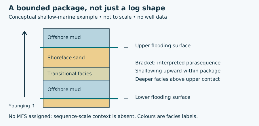
Worked interpretation: what does the column support?
Suppose an invented continuous core contains offshore mud, transitional facies and shoreface sand in that upward order, followed sharply by offshore mud. Assume the environmental labels have independent sedimentary-structure and fossil support and the section is upright. The upper contact is a candidate flooding surface. If a lower flooding boundary is also established, the intervening package is a candidate parasequence. The drawing supplies no thickness, duration, water-depth magnitude or regional correlation.
Now remove the environmental evidence and retain only “sand below mud.” The observed lithological change remains, but its flooding interpretation becomes less secure. Alternatively, retain all facies evidence but remove the lower contact through incomplete recovery: the top flooding interpretation may remain useful, while a complete bounded package cannot be demonstrated from this core alone. These are different uncertainties and should be recorded separately.
Carry the hypothesis into well correlation
Record the contact depth and its uncertainty, recovery and sample lag, then compare adjacent facies and other wells. A gamma-ray rise can help locate a change, but does not supply the missing environmental or regional evidence. Keep alternative correlations visible where samples are mixed or sections may be fault-repeated. Do not promote the largest local gamma-ray peak to maximum flooding simply because it is conspicuous. No pore-pressure, seal-capacity or reservoir-connectivity prediction follows from this schematic.
Concept references: SEPM Strata: Sequence Stratigraphic Framework; SLB definitions of flooding surface and maximum flooding surface. Original hypothetical example; no reproduced figure or expert review claimed. Compare oilfield terminology and facies migration; contact Chaser Geological for wellsite services.
Worked interpretation: is the coloured interval an ancient soil?
A paleosol records past soil formation. The USGS overview distinguishes buried, exhumed and relict examples. A soil horizon is a subdivision of a profile, not a synonym for a geological formation. The NRCS profile guide describes horizon properties and letter conventions.
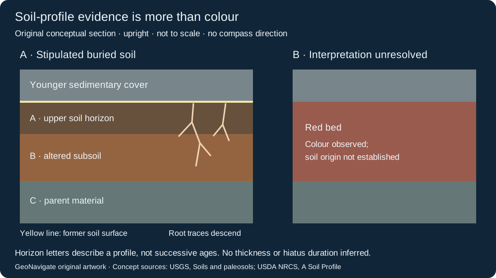
Case A: several observations support the interpretation
Invent an intact core with a younger sedimentary cover above a rooted interval. Roots branch downward from a common former surface. Below it, aggregate structure and a change in clay distribution organize the material into a profile. In this teaching case, independent examination has identified soil formation; the simplified A, B and C labels show its internal organization. They do not assign a soil order or climate.
Record each observation before interpreting it: contact character, roots and their point of origin, aggregate structure, mineral distribution, and changes with depth. Keep later veins and burial alteration separate. The profile crosses material that existed before the soil formed; reading its horizons as three successive depositional events would invent a history the observations do not supply.
Case B: colour is the only evidence
Invent a second core with a red bed but no preserved roots, profile organization or diagnostic soil structure. Record “red bed; origin unresolved.” The absence of those features does not prove that soil formation never occurred, but colour alone cannot distinguish soil development from other depositional or alteration histories. Do not correlate the two cores as one paleosol merely because their colours match.
Change the evidence: the upper profile is missing
If an erosional contact cuts the upper part of case A, retain the observed lower features and mark the upper profile as removed or unpreserved. Do not reconstruct its original thickness from this drawing. If roots instead originate in the younger cover and cut downward through the contact, they do not by themselves demonstrate rooting at the older surface. This change weakens that particular line of evidence.
The USGS discussion of loess paleosols notes that soil formation and sediment accumulation can occur together. A soil therefore does not automatically establish a long depositional gap or a synchronous regional marker. Compare independent stratigraphic evidence before assigning a hiatus or numerical age.
For a real example, the National Park Service describes the Yellow Mounds as soil-altered Pierre Shale preserved in the Badlands. That regional interpretation is not a colour template for another basin. At the wellsite, mixed cuttings may lose the contact and root geometry needed for this exercise; preserve sample provenance and seek intact core or outcrop evidence.
Original GeoNavigate explanation and artwork; sources checked 28 October 2026. No publication figure, measured core or external expert review is claimed. See the Oilfield Glossary, Geology Guides and Chaser Geological services.
Worked interpretation: which side of a cross-bed set is younger?
A dip measurement describes orientation, not stratigraphic order. Examine cross-bedding at its boundaries before assigning younging direction. The University of Alberta structural geology text emphasizes lamina truncation, which can survive deformation that changes lamina curvature. Its Banff example shows why horizontal-looking strata need not be upright.
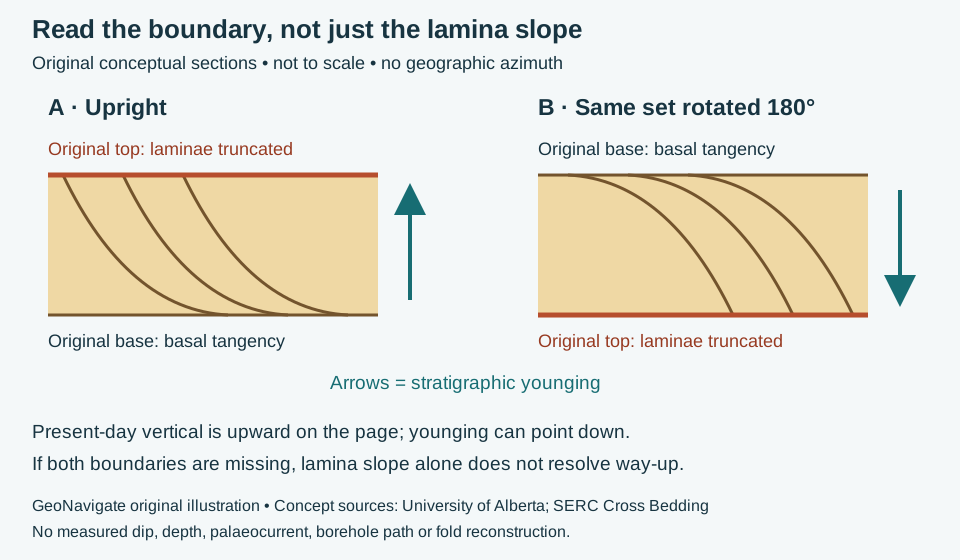
Two observations, then an interpretation
In invented panel A, inclined laminae terminate sharply against the upper set boundary and curve toward the lower boundary. The SERC cross-bedding teaching resource explains this common combination of erosional truncation and basal tangency. Once these are identified as primary depositional relationships, the original top lies toward the truncating boundary. The younging arrow points upward in the drawing.
Panel B rotates exactly the same geometry through 180 degrees. The original top now lies below the laminae in the present-day view. The younging arrow points down: the set is inverted. Rotation changes its orientation, not which material was deposited first. This example does not reconstruct a real fold or establish the orientation of an entire limb.
Change the evidence: the boundaries are missing
Suppose a narrow core piece contains only parallel inclined laminae. Neither set boundary survives. Record the observed lamina orientation, but leave way-up unresolved from that piece. Do not transfer panel A's interpretation merely because the lines slope in the same direction. A fracture cutting laminae is also not automatically a depositional truncation surface.
Apply the reasoning at the wellsite
This is an interpretation workflow, not a steering prescription. First retain the core run, sample order and orientation marks; verify that pieces have not been reversed during handling. Then compare several preserved set boundaries and independent indicators such as confidently identified normal grading. If observations disagree, retain the competing explanations rather than forcing a top pick. Mixed cuttings generally cannot preserve this bed-boundary geometry.
A younging observation does not by itself locate a thrust, prove repeated section, or distinguish regional overturning from local soft-sediment deformation. Combine it with mapped contacts, independent stratigraphic correlation and the well's surveyed trajectory. Gamma-ray similarity alone supplies neither the missing contact geometry nor a unique repetition diagnosis.
Original GeoNavigate exercise; sources checked 28 October 2026. No publication artwork or expert review claimed. Compare grading-based way-up, the Oilfield Glossary entry and Chaser wellsite geology services.
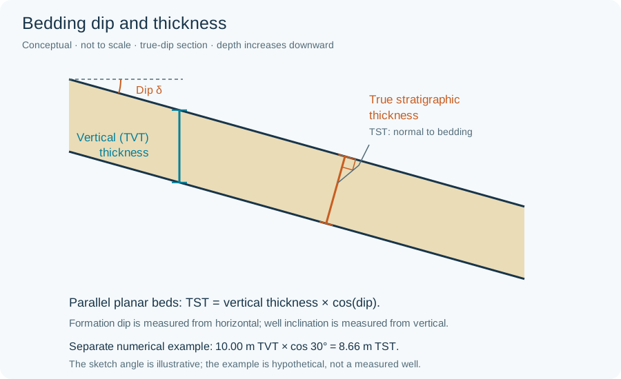
Worked measurement: apparent width is not lamina thickness
For invented parallel planar boundaries, a traverse measures 12 mm at 60° to the layer normal. True thickness is 12 × cos(60°) = 6 mm. Under the university text’s 1 cm convention, this is a lamina, despite its 12 mm apparent width. Compare the normal-versus-vertical thickness schematic. The 60° here is the traverse-to-normal angle, not formation dip. If orientation is unknown, retain apparent width and leave true thickness unresolved; do not assume this correction. This hypothetical geometry does not establish depositional duration or annual layering.
Fissility versus lamination: describe what splits and what changes
Lamination is fine layering; fissility is a tendency to split into sheets. They can occur together, but observing one does not demonstrate the other. In shale, splitting commonly follows bedding. Tectonic cleavage may cut across earlier layering. A single flat surface is insufficient to choose between them.
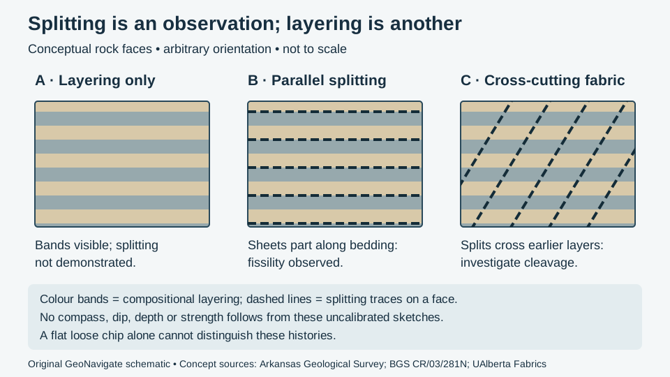
Worked interpretation: three invented observations
| Observation | Supported description | Still unresolved |
|---|---|---|
| A: intact fine-grained rock has alternating light and dark layers; repeated splitting has not been observed. | Laminated mudrock; fissility not demonstrated. | Whether the layers are mechanically weak. Absence of a split in one specimen does not prove its absence throughout the bed. |
| B: multiple sheets part along the same layering seen in intact material. | Fissile mudrock, with splitting parallel to observed bedding. | Mineralogy, strength, permeability and regional orientation. |
| C: repeated splitting surfaces cut the earlier layers at an angle. | A secondary planar fabric is a candidate; investigate tectonic cleavage. | Its mechanism and relationship to folds. A fracture set can require a different description. |
For an original counting exercise, imagine 20 randomly selected recovered chips: 12 show clear bedding-parallel splitting, 5 have visible layering but no demonstrated split, and 3 are too damaged to assess. Report 12/20 = 60% of the selected chips with the specified observation, plus both other categories. Do not call this 60% shale in the formation. The denominator is a chip count, not drilled volume, and recovery, fragmentation and preparation may bias it. Excluding the three damaged chips gives 12/17 ≈ 71% of assessable chips; that different denominator must be explicit.
Transfer the description to a wellsite record
Keep sample ID, collection time, assigned depth interval, lag basis and preparation together with the image. Photograph an intact face and a split face when available, with a scale and stated wet or dry condition. Identify which visible feature is layering and which is breakage. Loose cuttings do not retain the geographic attitude of their parent rock; camera-horizontal is not bedding-horizontal.
Use a change in fragment shape or fabric as a reason to compare adjacent samples, logs and drilling observations. It does not independently establish a fault, a repeated section, pore pressure or a safe operating limit. Distinguishing fresh drilled material from cavings, and distinguishing natural fabric from drilling or handling damage, remain separate interpretation steps. No strength or mud-weight calculation follows from this illustration.
Classification context and references
The mudstone entry uses the clastic, non-fissile sense; carbonate mudstone belongs to a different classification. State the scheme instead of applying a texture name without context. The references discuss different regions and purposes, so this exercise does not transfer their local rock properties to an Alberta formation.
- Arkansas Geological Survey: Shale — bedding-parallel fissility and the distinction from slaty cleavage.
- Merriman, Highley and Cameron (2003), BGS CR/03/281N — fine-grained rock descriptions; relevant report sections read, no figures copied.
- Waldron and Snyder, University of Alberta: Fabrics — fabric elements and secondary planar structures.
Sources checked 28 October 2026. The comparison and counting example are original educational synthesis, without an external expert-review claim. Continue to the Oilfield Glossary, Geology Guides, Chaser wellsite services or contact Chaser Geological.
Combined flow: reversal is not zero mean
Combined flow separates an oscillating component from a mean current. Hummocky cross-stratification is a preserved sedimentary geometry; do not treat either label as a direct measurement of the other.
Worked example: add two collinear velocities
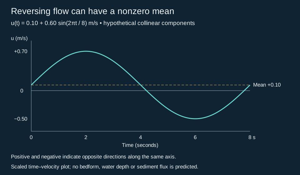
Stipulate u(t) = 0.10 + 0.60 sin(2πt/8) m/s. At 2 seconds the velocity is +0.70 m/s; at 6 seconds it is −0.50 m/s. Motion reverses, yet the cycle mean remains +0.10 m/s. Integrating this idealized velocity over eight seconds gives 0.80 m of signed displacement. That is a kinematic result, not a sediment-transport distance or flux: entrainment, settling, grain size and turbulence have not been modelled. For non-collinear waves and currents, add vector components instead.
Apply the distinction to rock descriptions
Experiments by Dumas and colleagues show that current strength and sediment accumulation affect preserved stratification. Their laboratory settings are not universal thresholds for interpreting every core. First describe lamina curvature, truncation, dip variation and the surrounding facies. A narrow core or detached cutting may not expose the lateral and three-dimensional relationships needed to confirm HCS. Keep a tentative interpretation separate from the observed structure; neither HCS nor a GR shape alone supplies a unique paleowater depth.
Sources: Dumas and Arnott (2006), Geology 34, 1073–1076 (text consulted via a university-hosted copy); Dumas, Arnott and Southard (2005), AAPG abstract. Original calculation checked 29 October 2026. See the oilfield context and wave ripples.
Average compass bearings across north without reversing the result
The existing imbrication example reverses one restored dip azimuth to infer a candidate flow direction. Averaging several dip measurements is a different operation. Compass bearings wrap at 360°; the pycircstat2 documentation describes averaging unit-vector components before converting back to an angle.
Worked example: 350° and 010°
Assume two equally weighted clast-surface dip azimuths, already restored to depositional bedding. Use north as 000° and increase azimuth clockwise. Their east components are sin(350°) and sin(10°), which cancel. Their north components are both cos(10°), about 0.9848. The mean vector therefore points north, at 000°. The ordinary arithmetic average, (350 + 10)/2 = 180°, points in the opposite direction and is inappropriate.
Only if an upstream-dipping fabric is supported does the next operation give candidate flow: (000° + 180°) modulo 360° = 180°. This does not establish the transport mechanism. The USGS-hosted Miao et al. study reports systematic observations of more than 2,000 clasts; the two-bearing exercise here is only arithmetic instruction.
Limits for geological reporting
Keep stratigraphic populations separate and retain the individual measurements. Opposed directions can cancel and leave no defined mean; a mean alone can conceal multiple populations. An undirected clast long axis has 180° ambiguity and must not be treated as a directed dip bearing. Loose cuttings cannot supply the original compass orientation. Record orientation provenance before using clast imbrication or paleocurrent interpretations in a report.
Worked example: find a median from sieve fractions
A median grain size (D50) locates the middle of a specified distribution. It does not describe the full spread. For this invented sieve analysis, use dry mass throughout, assume complete recovery of a 100 g prepared sample, and retain the fine fraction in the calculation.
| Fraction | Mass (g) |
|---|---|
| Passing 0.125 mm | 30 |
| Passing 0.25 mm, retained on 0.125 mm | 40 |
| Passing 0.50 mm, retained on 0.25 mm | 20 |
| Retained on 0.50 mm | 10 |
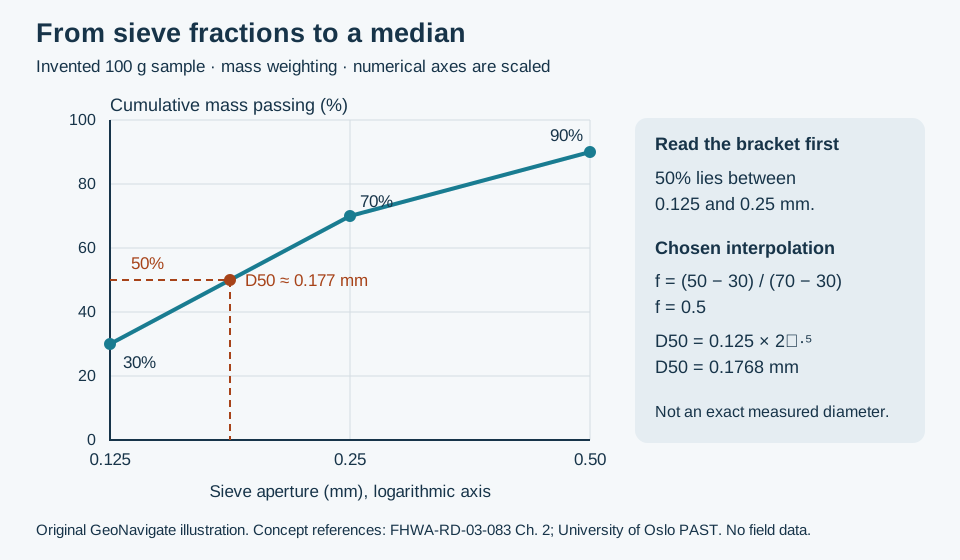
Mass balance is 30 + 40 + 20 + 10 = 100 g. Cumulative mass passing is therefore 30% at 0.125 mm, 70% at 0.25 mm and 90% at 0.50 mm. The 50% crossing lies inside the 0.125–0.25 mm interval. Without a model for sizes within that interval, the sieve results give a bracket, not an exact diameter.
Declare the interpolation before quoting a number
Here choose a straight cumulative segment against log diameter. The fractional distance to 50% is f = (50 − 30)/(70 − 30) = 0.5. Thus D50 = 0.125 × (0.25/0.125)0.5 = 0.1768 mm, approximately 0.177 mm. Equivalently, the endpoint phi values are 3 and 2, with an interpolated median of 2.5 phi. This equivalence follows from the logarithmic phi transformation.
Linear interpolation in diameter would instead give 0.1875 mm. That difference reflects a different within-bin assumption, not a second observation. Keep the original fractions so another reader can reproduce the chosen calculation. The open coarse and fine tails in this example do not locate the arithmetic mean, and a single median cannot assign a sorting class.
Use the represented population, not an implied formation population
If washing removed fines before weighing, the 100 g denominator describes only the recovered prepared material. Do not silently call its median the whole formation's median. Note sampling interval, preparation, loss and aggregation; distinguish liberated grains from cemented chips. Likewise, a number-weighted image median is a different statistic from this mass-weighted result. See the earlier count-versus-mass example.
This example estimates neither permeability nor a completion screen size. Those applications require additional measurements and context. Compare oilfield sieve-analysis terminology and the Chaser Geological wellsite services.
References checked 30 October 2026: FHWA-RD-03-083, Chapter 2 for mass-percent-finer notation and sieve methods; University of Oslo PAST grain-size documentation for fraction-weight inputs and statistical-method distinctions; USGS sieve-size analysis for method classification (indexed source text consulted). The masses, interpolation choice and drawing are original teaching material, not values from those studies.