
GEONAVIGATE / RESOURCES / GEOLOGICAL TIME
Geological time units: rocks versus time
Distinguish chronostratigraphic rock units from geochronologic time units, read their paired hierarchy and avoid common reporting errors.
Rocks and time need different words
A chronostratigraphic unit is a tangible body of rock representing a specified interval. A geochronologic unit is that interval of time. The paired names let a geologist say whether evidence concerns the material record or elapsed Earth history.
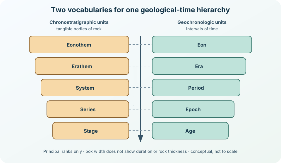
Read the pairs from large to small
| Rock body | Time interval | Relationship |
|---|---|---|
| Eonothem | Eon | contains erathems / eras |
| Erathem | Era | contains systems / periods |
| System | Period | contains series / epochs |
| Series | Epoch | contains stages / ages |
| Stage | Age | basic formal pair in this hierarchy |
These five principal ranks nest, but their durations are not equal. Subsidiary ranks, including subseries/subepochs and substages/subages, are omitted here. The diagram therefore uses box size only to communicate rank—not a time span, rock thickness or completeness of the local record.
A practical wording check
Suppose a report correlates a cored succession with rocks assigned to the Jurassic. “Jurassic System” refers to the rocks; “Jurassic Period” refers to the time during which those rocks formed. Likewise, a named stage is a rock unit and the paired age is time. In informal prose, “Jurassic rocks” and “during the Jurassic” are often clearer than forcing a formal unit name into every sentence.
A local gap is not missing time
An unconformity or hiatus can remove part of the rock record at one location. The corresponding interval still exists on the geological time scale. This is why a thin section does not imply a short duration, and why thickness should not be used as a substitute for time without an independently supported accumulation model.
What defines a boundary?
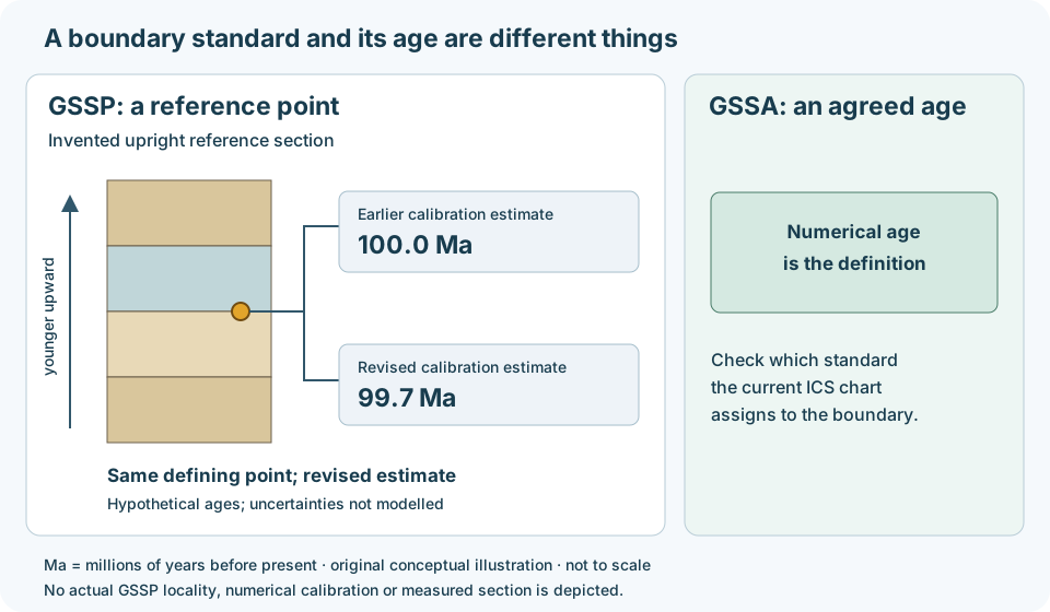
A GSSP fixes a boundary at a ratified point in a reference section. Its numerical age is a calibration that can improve with new evidence. A GSSA instead defines a boundary by an agreed numerical age. Do not apply the GSSP rule to every Precambrian boundary; check the current ICS chart.
Worked example: update the age, retain the reference
Imagine a boundary defined at a point in a reference section. An older calibration assigns 100.0 Ma; a later study estimates 99.7 Ma. The numerical estimate changes by 0.3 million years. That recalibration alone does not move the defining point. These deliberately invented values illustrate record keeping, not an actual boundary revision or a claim of precision.
In a well report, record the named boundary, the correlation evidence, the calibration source and its reported uncertainty separately. A local gamma-ray feature may support a tie, but a matching curve shape alone does not establish equivalence to the global boundary. Compare independent evidence and preserve uncertainty in the local pick. If the unit uses a GSSA, retain its agreed defining number rather than treating it as a replaceable calibration estimate.
Worked example: follow a rock boundary through time
A formation boundary follows a change in rock character. It may be diachronous: its age changes from place to place. An isochronous surface instead follows one time. The distinction matters when correlating wells across migrating depositional environments.
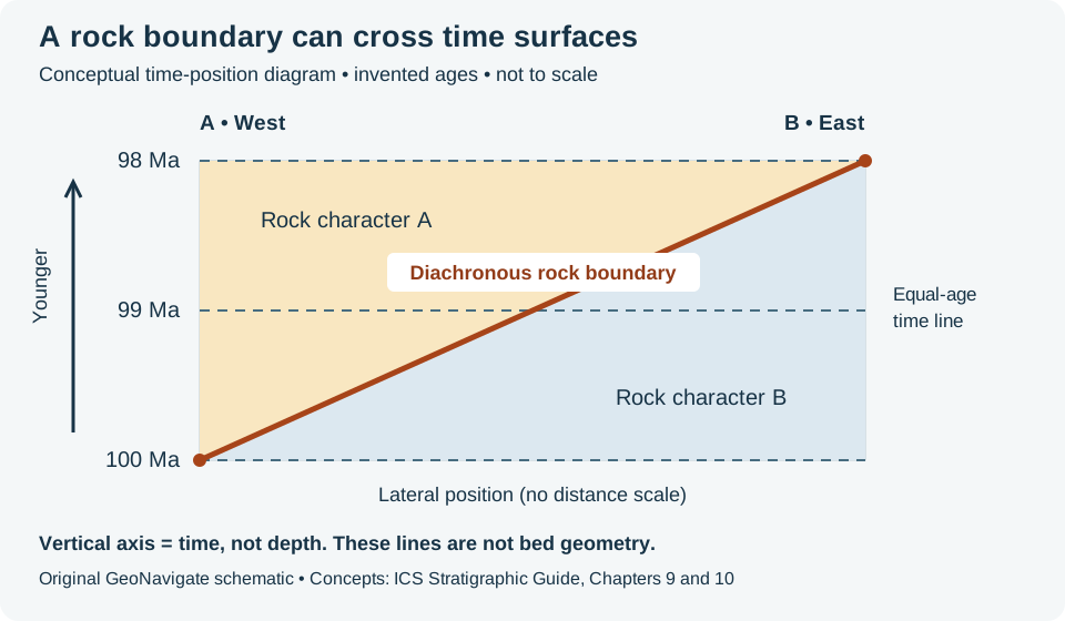
In this invented example, independent age evidence places the same traced rock boundary at 100 Ma in western section A and 98 Ma in eastern section B. Subtracting gives a two-million-year difference; the eastern pick is younger. A straight line between those picks crosses the 99 Ma time line. It therefore cannot also represent one instant everywhere. The connecting line is illustrative: it does not establish a constant migration rate, and the horizontal axis has no distance scale.
For a correlation panel, label the observed rock boundary and the inferred time tie separately. Record how each age was constrained and its uncertainty. Similar gamma-ray shapes can help identify a rock package; they do not by themselves supply the ages in this example. If age uncertainties overlap, report that the available evidence may not resolve a time difference instead of forcing an exact tie. A time-position plot also cannot give bed dip or thickness: neither axis here is depth.
Worked example: choose the bounding breaks
Imagine three beds between two mapped significant unconformities, with a brief depositional pause inside the middle bed. The outer surfaces could define a synthem, the basic formal kind of unconformity-bounded unit. The internal diastem is not an appropriate defining boundary under the ICS scheme. Trace the unit only where both bounding surfaces remain identifiable.
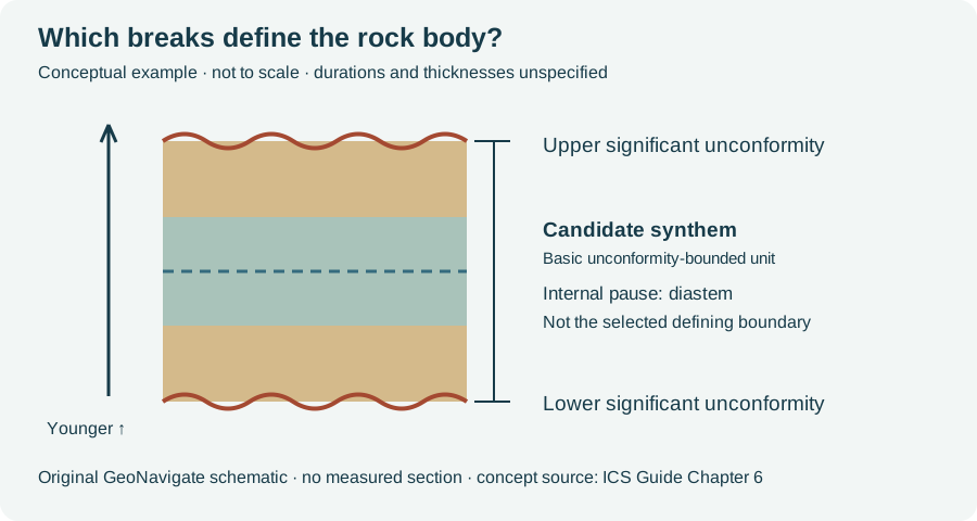
The hiatus is the time missing from the local succession; it is not a thickness that can be read directly from the drawing. For a well correlation, record each pick, the supporting observations and unresolved alternatives. Thickness alone cannot determine how much time a break represents. This invented sketch does not formally establish a unit or assign a numerical duration to either surface.
Sources and scope
- International Commission on Stratigraphy: Chronostratigraphic Units — definitions and paired hierarchy.
- International Commission on Stratigraphy: Principles of Stratigraphic Classification — tangible rock units versus intangible time units.
- International Chronostratigraphic Chart — current reference chart and downloads.
- USGS: Divisions of Geologic Time — paired terminology and North American usage.
Original explanation and vector artwork prepared 25 October 2026. No measured section, duration scale, reproduced chart or expert review is claimed. Continue with the Geology Dictionary, Oilfield Glossary, other geology guides, Chaser wellsite services or contact GeoNavigate.
A hiatus changes the time interval in an accumulation-rate calculation
Hiatus describes missing local sedimentary record, not time that stopped passing. ODP Leg 207 methods estimate sedimentation rates from age–depth relationships and discuss how breaks and uncertain age controls affect those estimates. The following original example makes the denominator explicit.
Worked model: 20 metres across four million years
Assume a hypothetical column accumulates 10 m during elapsed time 0–1 million years, nothing during 1–3 million years, then another 10 m during 3–4 million years. Stipulate no erosion, no compaction and a constant rate within each depositional interval. Elapsed time increases forward from an arbitrary start; it is not an age in Ma before present.
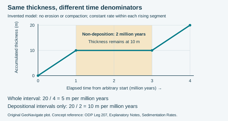
- Whole-interval average: 20 m / 4 million years = 5 m per million years.
- Average during deposition: 20 m / (1 + 1 million years) = 10 m per million years.
- Stipulated gap: 2 of the 4 million years has no deposition in this local model.
Both rates are correct for their stated denominators. Calling the first rate “the deposition rate” without qualification hides the pause. Dividing only by depositional time is justified here because that time is independently stipulated. If all that is known is 20 m between two age controls four million years apart, the endpoints alone cannot reveal a two-million-year hiatus or the active rate.
What changes in a real section?
Erosion can remove previously deposited thickness, and compaction can reduce preserved thickness; this plot includes neither. A preserved-thickness/time ratio then need not recover the original rate of sediment delivery. Keep thickness basis, dated horizons, uncertainties and evidence for missing record with the calculation. A lithological contact alone does not specify a hiatus duration. Compare unconformity, oilfield hiatus terminology and the bounding-break example above.
Source checked 31 October 2026: ODP Leg 207 Explanatory Notes, Sedimentation Rates. Arithmetic and plot are original, not measured well data or reproduced publication artwork. Chaser Geological services · Contact.