
GEONAVIGATE / RESOURCES / PALEONTOLOGY
Fossil preservation and reworking: interpreting age and evidence
Worked examples of fossil reworking, range-zone overlap, sample uncertainty, time averaging and trace-fossil evidence.
Separate the fossil from the age interpretation
A fossil description should identify what is preserved, the surrounding sediment and the evidence for its history. Body fossils preserve physical remains; trace fossils preserve activity. Neither label alone assigns a numerical age. Biostratigraphy uses fossil distributions through time, with identification and stratigraphic context essential to correlation.
One fossil can have more than one burial history
A reworked fossil leaves an earlier deposit and enters later sediment. The second host bed may therefore contain a fossil older than its own deposition. The schematic separates three events so that transport is not confused with the organism's lifetime.
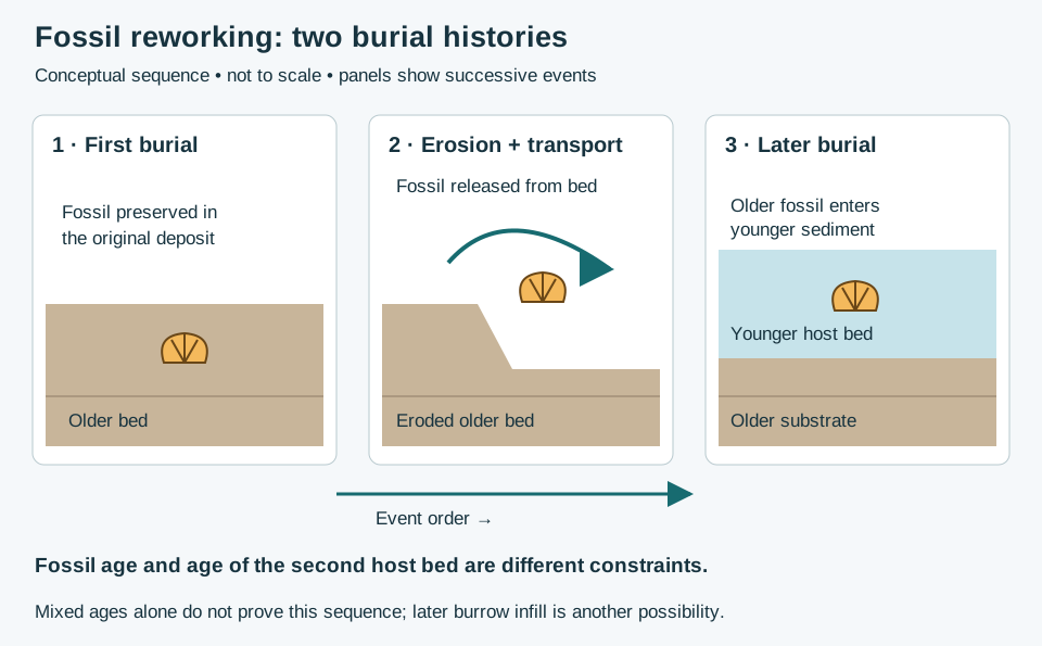
Check how the fossil entered the rock
The International Stratigraphic Guide separates erosion and redeposition from later introduction through burrows, root cavities or other pathways. For example, a younger fossil in burrow fill inside older sediment need not date the surrounding matrix. Record the fossil-bearing material and its contact with the host; mixed ages alone do not prove reworking. This geological introduction also differs from drilling cavings.
Worked example: why 100 Ma does not date the host bed
Consider a deliberately simplified teaching case: a fossil formed at 100 Ma, was eroded, and was redeposited at 80 Ma. Ma means millions of years before present; the larger number is older. The fossil is 20 million years older than its second burial. If only the fossil age is known, 80 Ma cannot be recovered from it alone. An independently established younger assemblage or other age constraint is needed to narrow the host-bed age.
Write “older fossil in younger host sediment; reworking interpreted from supporting evidence” when that evidence is available. If it is not, retain competing explanations instead of treating the numerical example as a field diagnosis. These ages are invented to illustrate the logic; they are not a dated sample or regional case study.
Preservation provides evidence, not a single-process answer
Taphonomy examines changes to remains. Decay, scavenging, transport and chemical alteration can affect preservation. Disarticulation means connected elements have separated. It does not uniquely demonstrate a long journey: decomposition can also separate bones. Record connectedness, breakage, abrasion and mineral alteration as distinct observations.
Build an interpretation that can be checked
- Record sample provenance and the observed host lithology. Keep specimen identifiers tied to the original sample record.
- Describe identification confidence and preservation before choosing an age interpretation.
- Compare multiple fossils and their positions. Look for an internally consistent assemblage and independently constrained stratigraphic order.
- Test mixing alternatives. Geological redeposition and disturbance introduced during sampling are different mechanisms; preserve the distinction in notes.
- State what would resolve the uncertainty: additional samples, specialist identification or independent dating evidence.
A USGS study of Horizon Guyot cores interpreted older Eocene fossils within younger assemblages as reworked, while considering bioturbation and sampling disturbance for younger material mixed downward. This is an example of evaluating context, not a rule that every mixed sample has the same origin.
Sources and scope
- National Park Service: Taphonomy — preservation processes and disarticulation.
- National Park Service: Fossils in Parks — body/trace categories and reworking.
- USGS: Fossil succession — fossil distributions and relative time.
- USGS Open-File Report 86-433 — Horizon Guyot core interpretation. Primary report text checked through indexed extracts; direct PDF retrieval was unavailable.
Original teaching example and vector illustration prepared 25 October 2026. No private well samples or reproduced publication figures. Continue with the Oilfield Glossary, Geology Dictionary or Chaser Geological wellsite services. Contact the team.
Worked example: zero recovery versus missing coverage
A barren interval concerns fossil content; a hiatus concerns missing time. Keep these interpretations separate.
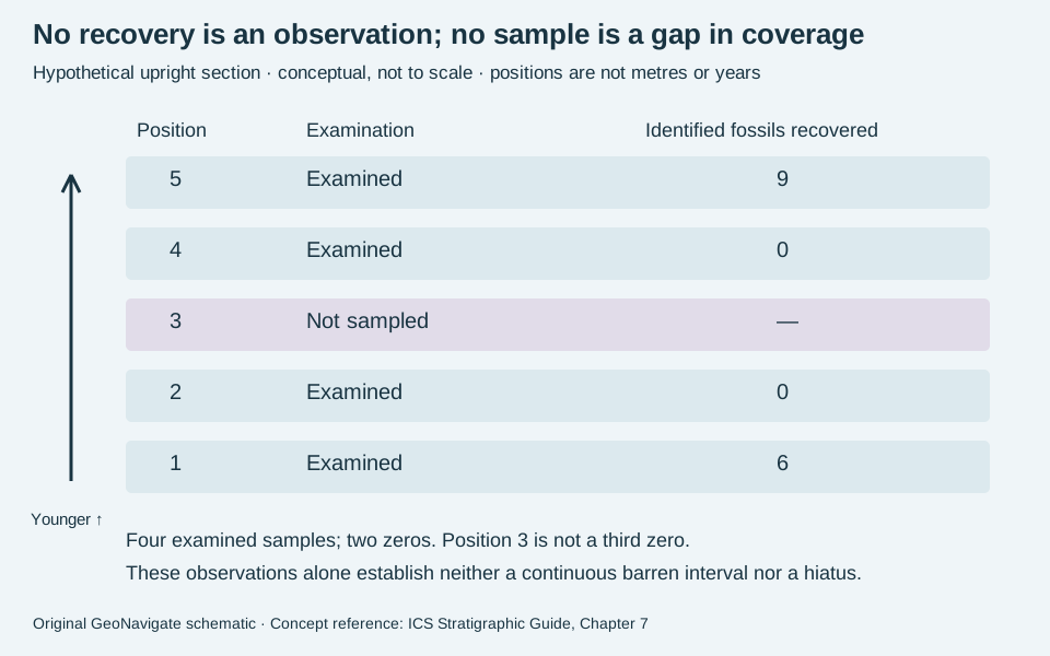
Count only the observations made
In an invented upright section, five positions run from older 1 to younger 5. Assume the same target fossil group and examination procedure for the four collected samples. Their recovered counts are 6 at position 1, zero at 2, zero at 4 and 9 at 5. Position 3 has no sample.
There are four examined samples and two zero-recovery results: 2/4 = 50%. Calling position 3 another zero would incorrectly give 3/5 = 60%. Neither fraction measures the proportion of the rock column that is fossil-free: sample positions have no assigned thickness or representative volumes in this exercise.
Write a defensible record
Report “no target fossils recovered from examined samples 2 and 4; position 3 unsampled.” Do not join the two zeros into a demonstrated continuous barren interval. Additional sampling could find fossils at position 3; even another zero would not prove absence everywhere between samples. Record preparation, material examined and identification limits before comparing results.
Do not infer erosion, non-deposition or an age merely from this ledger. Preserve lithological observations and independent age evidence alongside the fossil record. Compare the wellsite terminology and biostratigraphic classification.
Concept reference checked 31 October 2026: ICS Stratigraphic Guide, Chapter 7, sections B and C. Calculation, ledger and illustration are original teaching examples. Chaser Geological services.
Worked example: a lineage segment differs from the full range
A lineage biozone requires evidence that its taxa belong to an evolutionary succession. Merely finding different fossils higher in a section is insufficient. The evolutionary relationship in this exercise is an explicit assumption, not a conclusion drawn from the picture.
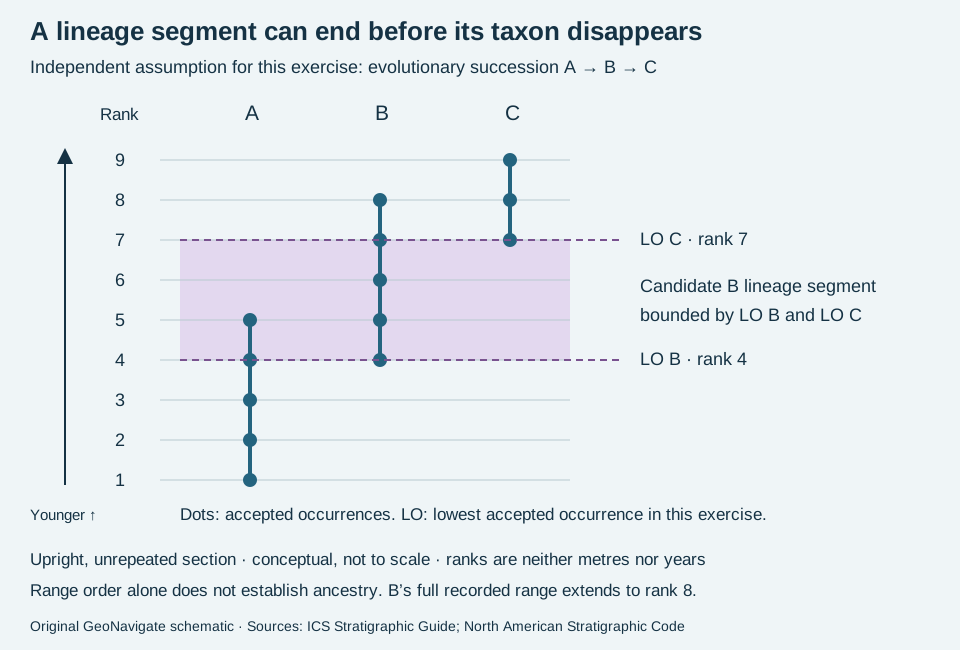
State what is observed and what is assumed
Invented accepted occurrences are A at ranks 1–5, B at 4–8 and C at 7–9. Assume that independent taxonomic and evolutionary work supports succession A to B to C. Define the lower boundary of the candidate B segment at lowest B, rank 4, and its upper boundary at lowest C, rank 7. B remains recorded above this boundary at rank 8. Thus the segment is not B’s complete taxon-range zone.
The boundaries are three rank steps apart. That gives neither a thickness nor a duration. The shared occurrence of B and C at ranks 7–8 also does not invalidate the exercise: the stipulated descendant’s appearance, not the predecessor’s disappearance, sets the upper boundary here.
Test the interpretation before using it for correlation
Without the independent lineage evidence, retain the observed ranges and describe the selected interval; do not call it a lineage zone solely because the lowest occurrences are ordered. If the lowest B sample is contaminated or C is misidentified, reassess the picks rather than silently shifting the data. In real sections, a lowest recorded occurrence may be limited by sampling or preservation and need not mark the taxon’s evolutionary origin.
For cuttings, document lag, identification and possible cavings before accepting occurrences. Preserve the sample record separately from lineage and boundary interpretations. Compare the Oilfield Glossary entry.
Sources checked 31 October 2026: ICS Stratigraphic Guide, chapter 7, lineage zones and North American Stratigraphic Code, Articles 50–51. Original hypothetical example and artwork; no private well data or expert review claimed. Chaser Geological services.
Worked example: a fossil association is not an abundance peak
An assemblage biozone uses a diagnostic association; an abundance biozone uses an elevated abundance. These are alternative criteria, not successive ranks. This exercise illustrates the distinction without establishing a formal zone.
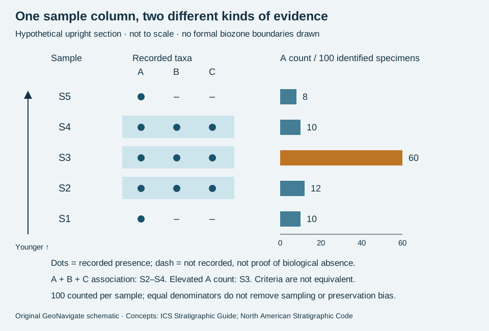
Read the invented observations
Count 100 identified specimens in each of five samples. From bottom to top, A counts are 10, 12, 60, 10 and 8. Taxa B and C are also recorded in S2, S3 and S4. The remaining specimens are other identified taxa; B and C counts are not individually specified. In this equal-denominator example, A percentages equal the stated counts.
If A, B and C form the independently established diagnostic association, S2–S4 supply assemblage evidence. The A abundance maximum is instead at S3: 60/100 = 60%, compared with 12% immediately below and 10% above. The observed association and peak therefore select different sample sets. No 60% universal threshold is implied, and this table cannot place boundaries within the unsampled intervals.
Keep recognition separate from correlation
Real assemblage-zone recognition need not require every diagnostic member in every sample. An abundance peak may reflect ecology, preservation or preparation, so matching two peaks alone does not establish a shared age. Record sample mass, size fraction, preparation, counting rules and taxonomic confidence before comparing counts. Equal totals alone do not standardize those factors.
For cuttings, first check cavings and reworked fossils. A dash in this schematic means “not recorded”; it is not an extinction event. Use additional samples and a stated reference framework before naming boundaries. Compare interval biozones and oilfield terminology.
Sources checked 31 October 2026: ICS Stratigraphic Guide, chapter 7 and North American Stratigraphic Code, Articles 50–51. Original hypothetical observations and artwork; no private samples or expert review claimed. Chaser Geological services.
Worked example: an interval without overlapping fossil ranges
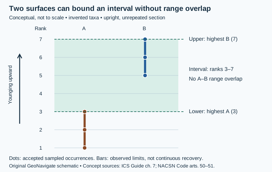
A biohorizon identifies a surface; an interval biozone identifies the strata between two chosen surfaces. The choice of boundary criterion matters. It cannot be recovered from two fossil names alone.
Specify both surfaces
In this invented section, accept indigenous taxon A at ranks 1, 2 and 3, and taxon B at ranks 5, 6 and 7. Other fossils occur in the intervening strata. Define the lower boundary using A’s highest accepted occurrence at rank 3 and the upper boundary using B’s highest accepted occurrence at rank 7. The candidate local interval runs from 3 to 7. It is neither A’s complete observed range nor B’s complete observed range.
By comparison, intersecting the two ranges gives a lower candidate limit of max(1, 5) = 5 and an upper candidate limit of min(3, 7) = 3. Because 5 exceeds 3, there is no concurrent-range zone for these two accepted ranges. This does not invalidate the separately defined interval. Four rank steps do not supply a thickness, duration or sedimentation rate.
Read a drilling record in its acquisition direction
Traversing this ideal section downward, B at rank 7 is encountered before A at rank 3. These first encounters downward are the highest accepted occurrences in the upright stratigraphic order. A missing sample would weaken the placement; it would not become evidence of fossil absence. In real cuttings, check cavings, lag and identification before accepting the picks. Keep the raw sample record alongside the interpretation.
Sources and limits
The International Stratigraphic Guide, chapter 7 defines biohorizons and discusses highest-occurrence interval zones in subsurface work. The North American Stratigraphic Code, Articles 50–51 distinguishes interval boundaries from range overlap. Both were read on 30 October 2026. These invented observations illustrate the distinction; they do not establish a formal regional zone or numerical age. Compare the Oilfield Glossary entry and Chaser Geological wellsite services.
From a fossil mould to a pore-system interpretation
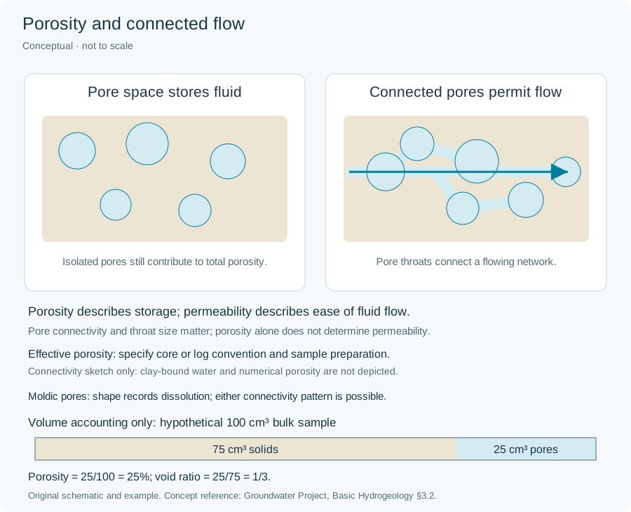
Moldic porosity forms when a constituent dissolves and leaves its shape as a cavity. The dissolved object need not be a fossil. SLB’s definition identifies pore origin; it does not establish connectivity. The Groundwater Project distinguishes interconnected pore volume from isolated or poorly exchanging space.
Worked volume ledger: stated assumptions matter
Consider a hypothetical 100 cm³ rock volume with 12 cm³ of moldic cavities and 8 cm³ of other pores. Stipulate that 3 cm³ of the moulds are completely isolated, all remaining pores are accessible to the chosen dry-core measurement, and no preparation-induced volume change occurs. Total porosity is (12 + 8)/100 = 20%. Connected porosity on this stated basis is (12 − 3 + 8)/100 = 17%. The 3-percentage-point difference comes from an assumed isolated volume, not from the appearance of a photograph.
If the isolated fraction is unknown, 17% cannot be inferred. Nor does the volume ledger predict permeability: throat geometry, network arrangement and direction still matter. This arithmetic is an original teaching example, not measured core data; log-based effective porosity may use a different clay-water convention. Compare the core/log porosity-basis example.
What belongs in a sample description?
Record cavity shape, visible fill and host lithology, with a scale and sample interval. A solid fossil cast occupies space that an empty mould would leave open. Broken chips can expose cavities that were enclosed in intact rock; describe the observation without assigning a connected-pore percentage or flow rate. Link the sample record to subsequent petrography or core measurements when available.
Mould, cast or steinkern: describe the preserved surface
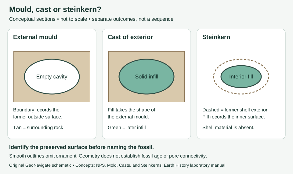
An external mould records an outside surface as an impression. Infilling can produce a cast. A steinkern instead records the shell interior. These distinctions concern preservation, not the age of the host bed. Sources: National Park Service definitions and Laboratory Manual for Earth History.
Worked observation exercise: two hypothetical chips
Assume chip A has a curved empty recess with fine ribs on its wall. Chip B contains a solid rounded body, but no outer ornament or enclosing shell is visible. A useful first description is “ribbed impression in chip A; solid rounded inclusion in chip B.” Interpretation can follow: A is consistent with an external mould, while B needs more evidence to distinguish a cast, a steinkern, or another grain. A smooth appearance alone does not establish an internal cast.
Photograph each chip with a scale, preserve its sample interval and describe the surrounding sediment. Examine a second view or broken face when available. Do not transfer a taxonomic identification from A to B merely because their outlines look similar. This is an original description exercise, not a measured well example or an identification key.
Use in wellsite reporting
Keep three observations separate: fossil shape, material occupying that shape, and visible void space. The terms fossil mould and fossil cast help make that record explicit. A sample photograph cannot establish connected pore volume or permeability; use the moldic-porosity entry for pore-system context. Before correlation, also consider the guide’s reworking and cavings comparison.
Reworked fossils and cavings: two different mixing histories
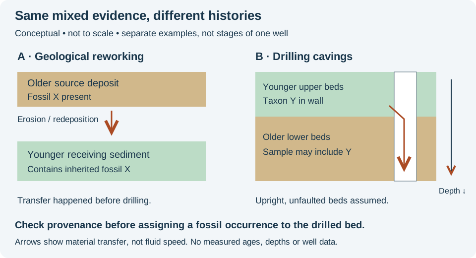
The International Stratigraphic Guide separates fossils eroded from older deposits and redeposited in younger sediment from indigenous fossils. That geological history differs from cavings added to a sample during drilling. A mixed sample does not by itself identify which process occurred.
Worked cuttings scenario
Imagine a vertical hole through an upright, unfaulted succession. Taxon Y is independently established in the upper, younger interval. Later, while drilling the lower, older interval, Y appears among its cuttings. One testable explanation is caving from the upper wall. Do not extend Y's depositional range downward solely from that occurrence. By contrast, an old fossil enclosed in a younger bed before the hole existed is a candidate for geological reworking.
In the AAPG applied-paleontology discussion by Fleisher and Lane, caving limits the reliability of lowest occurrences in cuttings. Keep first downhole encounter, lowest stratigraphic occurrence and evolutionary origin distinct. A downhole sampling sequence is not automatically a geological time sequence; overturning and fault repetition can change the age order.
Build an evidence record, not an automatic correction
- Keep sample interval, lag treatment, recovery method and laboratory identification with each occurrence.
- Compare the assemblage with earlier samples and the structural model; flag a possible source interval without silently deleting specimens.
- Use available intact core and independent stratigraphic constraints to test whether the fossil is within the host rock or introduced into the collected mixture.
For an invented count, 3 of 30 identified specimens are Y: 10% of that counted assemblage. It is not a 10% confidence estimate, a rock-volume fraction or a threshold proving contamination. If identification or provenance remains uncertain, retain the observation and qualify the interpretation.
Original teaching example, checked 28 October 2026; no private data or expert review claimed. Compare reworked fossil, oilfield cavings, and Chaser wellsite services; contact GeoNavigate for geological support.
Worked example: firmground or hardground?
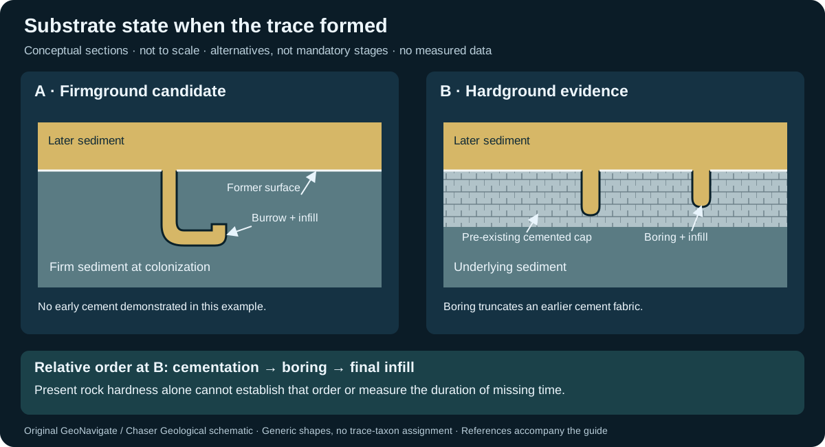
Describe the substrate as it was when a trace formed. A firmground was cohesive but unlithified; a hardground was already lithified. Present-day resistance to a hammer cannot establish that timing. The distinction matters when correlating omission or erosion surfaces in core.
Compare two hypothetical core contacts
| Contact | Observation | Working interpretation | Next check |
|---|---|---|---|
| A | Sharp-walled unlined burrows descend from a contact into compacted mud. Their sand fill resembles the overlying bed. | Candidate firmground colonization and later filling. | Check wall texture, earlier traces and evidence for cement present before burrowing. |
| B | A boring truncates a demonstrably earlier cement fabric at the exposed top of a carbonate bed. | Hard substrate existed before boring; a hardground interpretation is supported. | Verify the cement/boring relationship in thin section and distinguish in-place surface from a transported clast. |
At B, the observed cross-cutting order is cementation → boring → final infill. It establishes relative order, not elapsed time. At A, lack of visible cement in one section is incomplete evidence: retain “candidate firmground” until the substrate history is constrained. Record trace-fossil geometry and bioturbation separately from the environmental interpretation.
Do not turn one surface into a complete sea-level history
Trace assemblages reflect interacting substrate, oxygenation and sedimentation conditions. A named association is not a unique water-depth meter. The Betic carbonate study cited below combines trace evidence with sedimentology and tectonic relationships; its interpreted sea-level sequence cannot simply be assigned to every bored contact. A hiatus also needs independent constraints before it can be given a duration.
For a wellsite description, retain core position, contact relief, trace fill and cross-cutting notes with images at a recorded scale. Disaggregated cuttings may not preserve those relationships. A condensed section is a broader time–sediment interpretation; neither substrate label alone establishes its thickness or age range.
References checked 27 October 2026: University of Kansas Ichnology, Models; SEPM STRATA, Ichnofacies; Nieto and colleagues (2014), Betic unconformity surfaces. Original teaching case; no private core data or expert review claimed. See the Oilfield Glossary or contact Chaser Geological.
Time averaging: does one sample represent one community?
A death assemblage contains dead remains; a living census records organisms alive when surveyed. Fossil time averaging combines remains from different times. Even fossils touching on one bedding plane need not have lived together. Kansas Geological Survey describes how persistent shell concentrations and biological sediment mixing can blur these distinctions. Pooling several sampled beds can introduce additional mixing.
Worked example: count and time are different observations
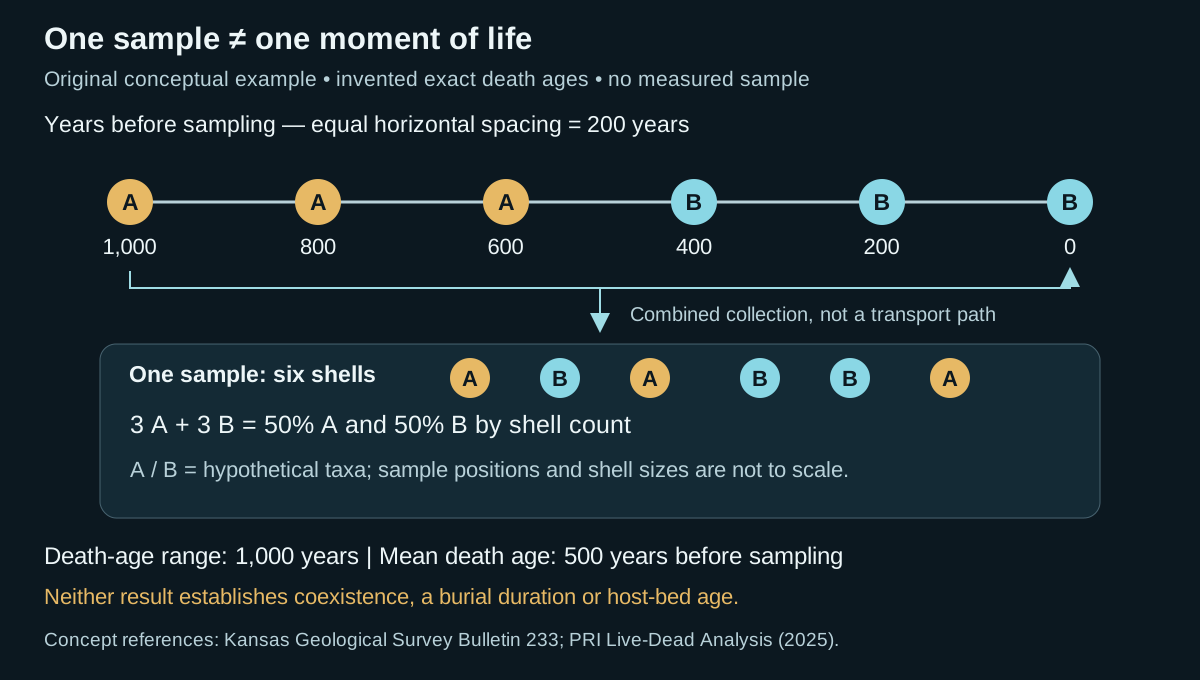
Suppose six identifiable shells have independently established death ages of 1,000, 800, 600, 400, 200 and 0 years before sampling. Zero denotes the sampling reference time, not a geological era boundary. For this arithmetic exercise only, treat the ages as exact. Assign hypothetical taxon A to the first three shells and B to the last three. The combined collection contains three A and three B: 50% of each by shell count.
The observed death-age range is 1,000 − 0 = 1,000 years. The arithmetic mean is 3,000/6 = 500 years before sampling. No listed shell died at that mean time. Neither the mean nor the equal counts demonstrate a living community containing 50% A and 50% B. Death dates do not supply lifespans, and the example does not establish whether individuals overlapped in life.
Those numbers also do not date deposition of a host bed. Burial histories and sampling context are unspecified. A rapid event could gather remains with differing death ages; the duration of that event is a separate question. The Digital Atlas of Ancient Life illustrates this distinction with marine shell accumulations. Real dating uncertainty, preservation losses and uncollected specimens make the six-shell calculation an incomplete estimate of a natural assemblage's history.
What to retain in core and wellsite notes
- Keep observed taxon counts separate from age estimates and inferred environments. State whether a count refers to shells, valves, fragments or reconstructed individuals.
- Record the sampled interval and intact sedimentary relationships. Do not treat pooled cuttings as a single bedding-plane assemblage.
- Describe abrasion, disarticulation and mixed preservation without assigning a unique duration to any one feature.
- Evaluate geological reworking, natural sediment mixing and collection-induced mixing separately. Seek independent stratigraphic and age constraints before using the assemblage for correlation.
Time averaging does not make a collection useless. Kidwell's 2013 review describes how modern death assemblages can retain regional ecological information over longer intervals than a living census, especially in studied marine molluscan settings. That potential does not justify transferring every result to an unrelated fossil group or depositional setting.
Sources and scope for this example
- Roger L. Kaesler, Kansas Geological Survey Bulletin 233: Ancient communities in the fossil record — time averaging and sampling resolution.
- Goben and colleagues (2025), Paleontological Research Institution: Live-Dead Analysis — living versus death assemblages.
- Digital Atlas of Ancient Life: The process of fossilization — marine shell accumulation and temporal association.
- Susan M. Kidwell (2013), Time-averaging and fidelity of modern death assemblages, DOI 10.1111/pala.12042 — publisher abstract checked; no full-paper review claimed.
Original GeoNavigate example and artwork; sources checked 27 October 2026. No external expert review claimed. See the Oilfield Glossary definition, Geology Guides, Chaser Geological wellsite services or contact Chaser Geological.
Reading burrowed sediment: fabric, index and environment
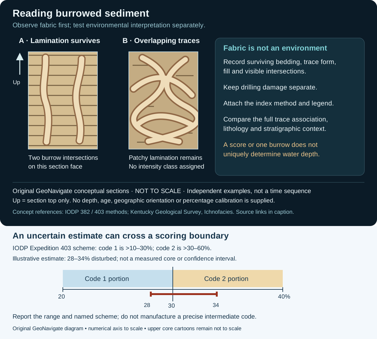
Start with what is visible. Ichnofabric describes the preserved effects of biological activity within sediment; ichnofacies interprets an association of traces in an environmental framework. A numerical intensity class is neither a species identification nor an environment. The distinctions matter when comparing core descriptions from different projects.
Worked example: two logs both say “3”
Imagine two inherited core logs whose only shared field is an intensity value of 3. In the scheme documented for IODP Expedition 382, 3 represents moderate biological reworking of 10–40% of the observed surface. In the scheme documented for Expedition 403, 3 represents heavy reworking, greater than 60% and up to 90%. These reported ranges do not overlap. Equal codes therefore do not establish equal fabric.
This is an invented comparison using two real method legends, not a comparison of sampled expedition cores. Preserve each original value, source method and observation basis. If a common reporting category is needed, return to the observations or images and document the new classification. Simply subtracting one from every code or rescaling the maximum would discard the category meanings. Percentages of a visible surface also should not silently become percentages of a three-dimensional sediment volume.
Describe the evidence before naming the environment
- Record core identifier, sampled interval, depth convention, exposed face and image scale. Describe lamination that survives between traces, rather than treating a missing structure as automatically destroyed by organisms.
- Describe trace shape, fill, orientation relative to bedding and visible intersections. Keep an uncertain identification explicit. The unlabelled burrow shapes in this teaching sketch are not diagnostic ichnotaxa.
- Separate possible drilling damage from bioturbation. Expedition 382 records coring disturbance separately; deformation or mixing alone is insufficient to establish a biological origin.
- When assigning an intensity score, attach the named method and legend. Record the observations behind the score so another reader can reassess it.
- Evaluate the whole trace association alongside sedimentary structures and stratigraphy. Kentucky Geological Survey explains that oxygenation and other controls can produce similar associations at different water depths. An isolated burrow or score cannot resolve that ambiguity.
A useful reporting statement
For the left-hand sketch, a defensible teaching description is “horizontal lamination preserved between two schematic burrow intersections; ichnotaxa and intensity class unassigned.” It does not claim a burrow count for the entire bed, identify the producer, establish oxygen concentration or determine water depth. In an actual wellsite report, retain the evidence that would support each added interpretation.
Intact core preserves relationships that loose fragments may lose. Describe the observation scale: an apparent vertical burrow on one cut face is not a complete three-dimensional reconstruction. A conceptual illustration cannot calibrate a percentage estimate in a real sample.
Sources and scope
- IODP Expedition 382 methods, Bioturbation and Core disturbance sections: separate fabric, index and drilling observations.
- IODP Expedition 403 methods, §2.5.5: the alternative intensity legend used in the comparison.
- Kentucky Geological Survey: Ichnofacies: environmental controls and the Borden Formation example. Archived educational page; not a current regional assessment.
Original GeoNavigate explanation and vector artwork; sources checked 27 October 2026. No private well data, reused artwork or external expert-review claim. Continue with the Oilfield Glossary, Geology Guides, Chaser Geological wellsite services or contact Chaser Geological.
Worked example: uncertainty at an ichnofabric boundary
The named scoring scheme is only the first part of a defensible ichnofabric record. Also preserve how confidently the observed fabric fits its categories. For this example, use the IODP Expedition 403 methods, §2.5.5: code 1 covers a disturbed fraction greater than 10% through 30%; code 2 covers greater than 30% through 60%. These limits belong to that scheme, not every bioturbation scale.
Imagine that ambiguous burrow margins lead you to estimate 28–34% disturbance on one defined observation surface. This is an invented plausible range, not a statistical confidence interval. It straddles 30%: values from 28% through 30% fit code 1, while values above 30% through 34% fit code 2. The evidence therefore supports a boundary qualification rather than an unqualified code.
A record that retains the evidence
For the invented observation, a useful note is: “Disturbance estimated at 28–34% on the described surface; Expedition 403 scheme, code 1/2 boundary; ambiguous margins retained in the estimate.” If a database requires one integer, document the chosen project rule and keep the original range alongside it. A midpoint of 31% would fall in code 2, but selecting that midpoint does not remove the observational uncertainty.
Do not turn codes 1 and 2 into an assumed measurement of 1.5, infer probabilities from the length of the range, or interpret an environmental change merely because two uncertain observations fall on opposite sides of the threshold. Reinspect surviving lamination, burrow geometry and possible drilling disturbance. An ichnofacies interpretation still needs the trace association and geological context.
Source checked 31 October 2026. Original teaching example and artwork; no measured core, reproduced publication figure or expert review claimed. See the Oilfield Glossary entry, Chaser Geological services or contact Chaser.
Worked example: reading fossil ranges without inventing an age
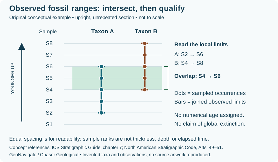
Two fossil names in one bag do not yet establish a reliable correlation. First separate the sample observations from the ranges drawn through them. This exercise uses invented taxa A and B in eight ordered samples from a stipulated upright, unrepeated section. Sample labels are ranks, not metres, drilling depths or equal durations.
Keep the observations explicit
| Taxon | Positive sample identifications | Local observed limits |
|---|---|---|
| A | S2, S3, S4, S5, S6 | S2 to S6 |
| B | S4, S5, S6, S7, S8 | S4 to S8 |
For this exercise, accept each identification and assume the specimens belong to the enclosing deposit. The local expression of A’s taxon-range zone extends from S2 to S6. That statement summarizes this section; it does not establish A’s first evolution or final extinction anywhere on Earth.
Intersect the ranges
The candidate local concurrent-range zone begins at S4, where the later-starting B is first observed upward, and ends at S6, where the earlier-ending A is last observed upward. In rank arithmetic, the lower limit is max(2, 4) = 4 and the upper limit is min(6, 8) = 6. Both taxa occur at S4, S5 and S6 in the stipulated observations. Three sampled levels do not mean three metres or three million years.
The overlap is shorter than either individual observed range here, but its numerical age remains unknown. A formation contact is not required to coincide with either end. Across another section, matching this fossil criterion provides a biostratigraphic comparison; establishing a particular time surface needs additional evidence.
Change the evidence and revise the range
Suppose examination shows that the A specimen at S6 was redeposited from older sediment. Retain the specimen record, but exclude it from the accepted indigenous occurrences used here. A’s highest accepted occurrence becomes S5, and the observed overlap contracts to S4–S5. This changes the local evidential limit; it does not prove that A became extinct at S5.
Alternatively, keep the original identifications but remove sample S5 entirely. A and B remain documented at S4 and S6. A connecting bar may summarize their observed endpoints, but it cannot turn the unsampled S5 level into a positive observation. Show the missing sample rather than replacing it with either a fossil occurrence or a demonstrated absence. No sedimentation rate can be calculated from these sample ranks.
Transfer the reasoning to wellsite records
The same range logic can be applied to appropriately identified palynomorphs. Preserve the taxon, sample interval, identification confidence and mixing interpretation. In cuttings, first encountered while drilling downward differs from lowest stratigraphic occurrence; caving and recirculation can introduce material from previously drilled strata. A repeated structural section would also invalidate the stipulated simple order. Resolve those alternatives before extending an apparent range.
References and scope
Definitions and cautions checked 28 October 2026 against the International Commission on Stratigraphy’s Stratigraphic Guide, chapter 7 and North American Stratigraphic Code, Articles 49–51. These are original hypothetical observations, arithmetic and artwork, not a regional zonation or measured well result. No external expert review is claimed. Compare the Oilfield Glossary explanation, Chaser Geological wellsite services or contact Chaser Geological.