Mineral–melt partitioning: concentration, compatibility and mass

Write the phase order before calculating

A mineral chemistry result and a whole-rock analysis describe different materials. To calculate a mineral–melt partition coefficient, compare the same element in a specified mineral and its coexisting melt at equilibrium: K = C_mineral / C_melt. Use matching concentration units and basis. This guide uses mass concentrations in mg/kg (equivalent to ppm by mass). Symbols vary between references; the written ratio removes that ambiguity.

Compatible means K > 1 for this pair; incompatible means K < 1. K = 1 means equal concentrations. These are relative properties, not permanent labels independent of mineral and melt.

Worked example: a ratio is not a percentage

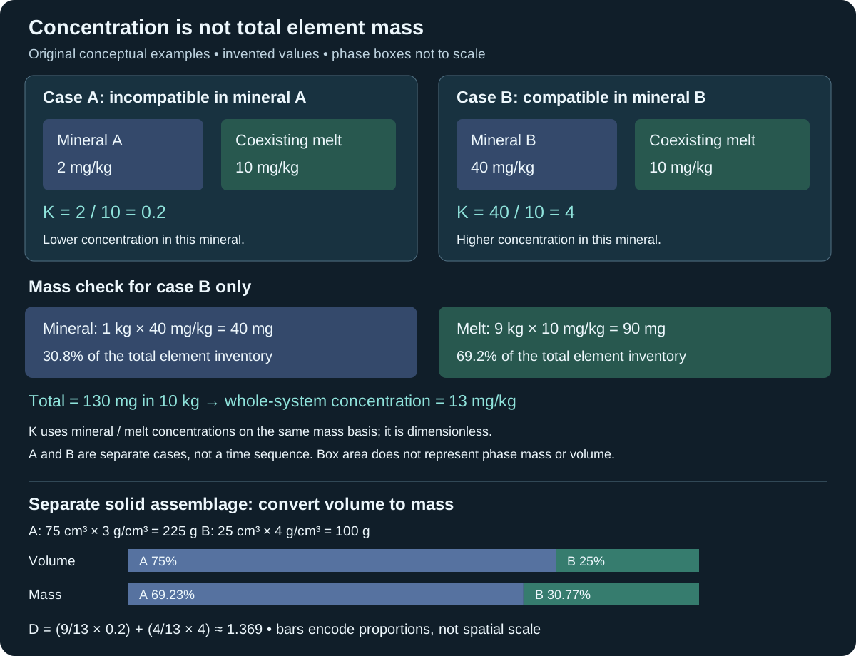
Assume two separate hypothetical equilibrium experiments. In case A, mineral concentration is 2 mg/kg and melt concentration is 10 mg/kg: K = 2/10 = 0.2. The element is incompatible in mineral A. This does not mean that 20% of all element mass is in the mineral.

In case B, mineral concentration is 40 mg/kg and melt concentration is 10 mg/kg: K = 40/10 = 4. The element is compatible in mineral B. Writing melt/mineral instead would give 0.25, so always check phase order before applying the threshold. The two cases do not represent successive stages of one magma.

Worked mass check: where is the element?

Let case B contain 1 kg of mineral and 9 kg of melt. Multiply each concentration by its phase mass:

• Mineral inventory: 40 mg/kg × 1 kg = 40 mg.
• Melt inventory: 10 mg/kg × 9 kg = 90 mg.
• Total: 130 mg in 10 kg, giving a whole-system concentration of 13 mg/kg.

The mineral contains 40/130 = 30.8% of the element inventory, rounded, despite having four times the melt concentration. The remaining 69.2% is in the melt. Substituting the 13 mg/kg whole-system value for the 10 mg/kg melt value would produce 40/13 = 3.08, which is a different ratio and is not the specified mineral–melt coefficient.

An assemblage needs mineral proportions

For coexisting minerals, a bulk solid/melt coefficient is a mass-weighted sum of the individual coefficients. The fractions refer to the solid assemblage and sum to one. In a separate invented example, 75% mineral A with K = 0.2 and 25% mineral B with K = 4 give D = 0.75 × 0.2 + 0.25 × 4 = 1.15. A plain average would give 2.1 and would assume equal mineral masses. This calculation is an assemblage average, not an estimate of melt fraction or a crystallization path.

Worked example: volume proportions are not mass fractions

Consider a separate hypothetical solid assemblage: 75 cm³ of mineral A at density 3 g/cm³ and 25 cm³ of mineral B at 4 g/cm³. Their masses are 225 g and 100 g. Thus the mass fractions are 225/325 = 9/13 and 100/325 = 4/13, approximately 69.23% and 30.77%.

With the illustrative coefficients K_A = 0.2 and K_B = 4, the mass-based bulk coefficient is D = (9/13 × 0.2) + (4/13 × 4) = 1.369, rounded. Inserting volume fractions directly gives 1.15 instead. That earlier result is correct for 75:25 mass proportions, a different assemblage.

In general, f_i = ρ_iV_i / Σρ_jV_j. Normalize over the solid minerals only; do not include melt in these fractions. State whether measured modes describe volume or mass, and use appropriate mineral densities. Equal densities make the two sets of fractions coincide. These invented densities and coefficients are not assignments to named minerals or a melting-path model.

From an analysis to a defensible interpretation

1. Identify the analysed phase and element. Keep crystal, glass and whole-rock results separate; report units, analytical uncertainty and detection limits.
2. Establish whether the mineral and melt genuinely coexisted and approached equilibrium. A convenient ratio between unrelated samples is not an equilibrium coefficient.
3. Retain the experimental or geological conditions associated with a published coefficient. Changing mineral or melt composition can change the result; do not assign the invented A/B values to feldspar or any named mineral.
4. Record mineral proportions when calculating an assemblage value. Keep model assumptions separate from observed chemistry.

At the wellsite, mixed cuttings are not a preserved equilibrium mineral–melt pair. Sample mixing and preparation must be assessed before comparing laboratory chemistry. Use the glossary definition and mineral-identification guide to keep observations distinct from a petrogenetic interpretation. A single coefficient does not establish a magma source, formation correlation or reservoir property.

References and authorship

Original GeoNavigate explanations, arithmetic and artwork. Sources checked 27 October 2026; no external expert review claimed. No private well data or reproduced figures are included.

• Imperial College London, ESE Jupyter Material: Distribution coefficients — phase ratios, equilibrium and bulk mass weighting.
• Peate & Hawkesworth (2005), U series disequilibria, section 2.4.1 — mineral/melt compatibility and composition dependence; DOI 10.1029/2004RG000154.
• Stephen A. Nelson, Tulane University: Magmatic differentiation — geological context and alternative causes of chemical variation.

Explore more geology guides, Chaser Geological services, or contact Chaser Geological.

When does an assemblage become compatible?

A mineral coefficient and a bulk solid coefficient answer different questions. The Imperial College distribution-coefficient notes define the bulk coefficient as a sum weighted by mineral mass fractions. Changing those fractions can change the bulk classification without changing either mineral coefficient.

Work out the crossover

Consider hypothetical coexisting minerals A and B, with fixed coefficients K_A = 0.2 and K_B = 4 for one element and the same melt. Let f be B's fraction of the solid mass; A's fraction is 1 − f. Then D = 0.2(1 − f) + 4f = 0.2 + 3.8f. Setting D = 1 gives f = 0.8/3.8 = 4/19 ≈ 0.210526, or about 21.05% B by mass.

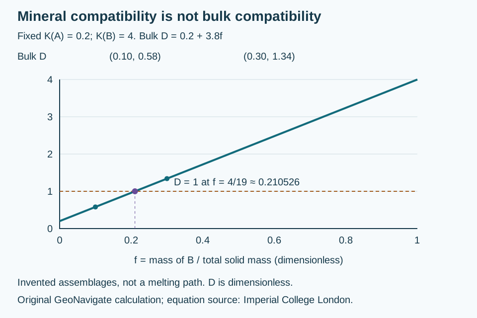
At f = 0.10, D = 0.58: the element is bulk-incompatible even though it is compatible in B. At f = 0.30, D = 1.34: it is bulk-compatible even though it remains incompatible in A. At the crossover, the bulk solid and melt have equal concentrations; this does not require equal element inventories because their total masses may differ.

Keep the basis and assumptions visible

The denominator in f is the mass of all solid minerals, not the mass of solids plus melt. Thus f is neither melt fraction nor the proportion of the element held by B. If the measured proportions are volumes, first use the density conversion above. Coefficients, mineral proportions and phase stability can change in real magmas; the line compares stipulated assemblages and is not a crystallization trajectory.

Report whether compatible or incompatible refers to a particular mineral or the whole solid assemblage. A classification based on an assumed assemblage does not identify a source rock from mixed cuttings. Original arithmetic and artwork, checked 31 October 2026. No private samples or external expert review claimed. See the Oilfield Glossary and Chaser Geological services.

Melting versus crystal removal: two mass-balance examples

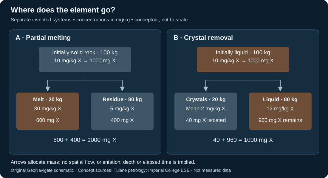
Partial melting leaves solid residue while producing liquid. Fractional crystallization isolates crystals from the remaining melt. The Tulane petrology notes explain both processes. The two invented systems below start with the same mass and element inventory, but their starting materials and histories differ. They are not successive stages of one magma.

A. Partial melting of an initially solid source

Take 100 kg of rock containing element X at 10 mg/kg: the inventory is 1000 mg. Stipulate 20 kg of melt at 30 mg/kg and 80 kg of residue at 5 mg/kg. The inventory check is 20 × 30 + 80 × 5 = 600 + 400 = 1000 mg. The melt holds 60% of the element in 20% of the system mass. Its concentration is three times the initial whole-rock concentration; neither number is the fraction of rock melted.

For an equilibrium batch model, define F as melt mass divided by initial mass and D as bulk residual-solid concentration divided by melt concentration. Then C₀ = FCₗ + (1 − F)Cₛ and Cₗ = C₀/[F + D(1 − F)]. Here F = 0.20 and D = 5/30 = 1/6; the equation returns 30 mg/kg. This follows the Imperial College London batch-melting model. It assumes retained melt and solid equilibrate; continuous melt extraction is a different model.

Change only the assumed F to 0.50 while holding C₀ = 10 and D = 1/6 fixed. The model gives Cₗ = 120/7 ≈ 17.14 mg/kg and Cₛ = 20/7 ≈ 2.86 mg/kg. Two 50 kg portions still sum to 1000 mg. Real mineral proportions and D may change during melting, so this is a sensitivity calculation, not a temperature or source-rock prediction.

B. Removal of crystals from an initially liquid system

Start a separate 100 kg liquid containing 10 mg/kg of X. Stipulate that the accumulated 20 kg of isolated crystals has a mass-weighted mean concentration of 2 mg/kg. It removes 40 mg of X. The remaining 80 kg must hold 960 mg, hence 12 mg/kg. Mass conservation determines this result without identifying the crystals or prescribing a cooling path.

The 2 mg/kg is an average of the removed material; dividing it by the final melt value does not recover an instantaneous equilibrium coefficient. This single removal budget is not a fitted continuous Rayleigh crystallization model. If the removed crystals instead averaged 20 mg/kg, they would remove 400 mg and the remaining liquid would contain 600/80 = 7.5 mg/kg. Removal can enrich or deplete the remaining liquid depending on what is taken away.

Test the interpretation beyond the budget

In their 2010 mid-ocean-ridge dacite study, Wanless, Perfit, Ridley and Klein found that fractional crystallization alone did not explain the geochemical signature; crustal melting and assimilation also mattered. The USGS record and abstract provide this example; DOI 10.1093/petrology/egq056. It is not a regional calibration for our invented X.

Keep analysed glass, individual crystals and whole-rock compositions separate. Retain sample relationships, uncertainty and possible alteration before interpreting an igneous history. A matching budget is necessary but does not uniquely identify the process. For migmatite, field and petrographic evidence must establish which components represent melt and residue; this diagram is not a texture-identification key.

Original GeoNavigate explanation, arithmetic and vector artwork; source concepts checked 28 October 2026. No measured data, copied publication figure or external expert review is claimed. Compare the oilfield definition, explore Geology Guides, or contact Chaser Geological.