Capillary entry pressure: a pore-throat worked example

State which pressure is being subtracted

Capillary pressure is a difference between fluid pressures, not the absolute pressure of a reservoir. This guide uses Pc = Pnonwetting − Pwetting. In the water-wet example below, water is the wetting fluid. A different fluid ordering reverses the sign; a software parameter called suction may use another convention.

A small throat can set the entry threshold

A pore body can store fluid but access depends on its connecting throats. An ideal cylindrical throat gives Pc = 2γ cos θ / r, where γ is interfacial tension in N/m, θ is measured through the wetting fluid, and r is throat radius in metres. This is a geometric teaching model, not a complete rock pore network. Wettability and fluid properties must accompany any radius estimate.

Worked example: same fluids, different throat

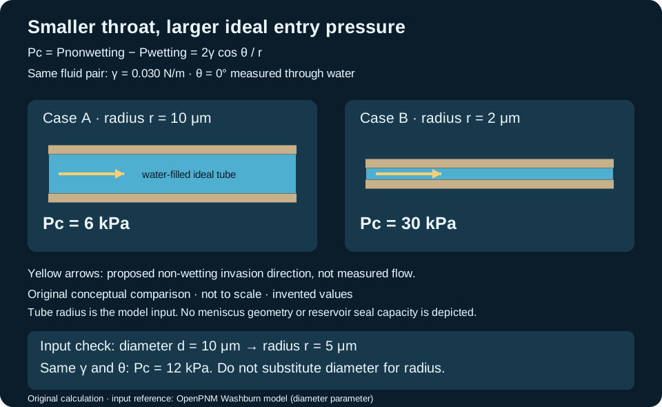
Use invented values γ = 0.030 N/m and θ = 0°, so cos θ = 1. At r = 10 μm = 0.000010 m, Pc = 2 × 0.030 / 0.000010 = 6,000 Pa = 6 kPa. At r = 2 μm, Pc = 30,000 Pa = 30 kPa. Reducing radius fivefold raises the ideal threshold fivefold. These are pressure differences; neither result specifies burial depth.

Check sensitivity before interpreting a rock

For the 10 μm throat, changing θ from 0° to 60° while holding γ fixed halves the calculated threshold to 3 kPa. Changing γ to 0.015 N/m at θ = 0° also gives 3 kPa. This arithmetic shows why a laboratory result cannot be transferred between fluid systems using pore geometry alone. Specify the angle convention and fluid pair before comparing numbers.

What this calculation cannot tell you

The example represents one accessible tube. It does not determine the connected invasion path through a core, predict relative permeability, or establish a seal's field capacity. Record sample condition, test fluids and displacement history alongside measured pressure–saturation data. Keep an inferred geometric radius distinct from an independently imaged throat.

Gravity drainage also leaves water behind on surfaces and within pore spaces. Thus connected pore volume is not automatically recoverable water volume: specific yield describes the amount released per bulk sample volume, and that measured amount depends on drainage time. This is one reason a porosity description alone is insufficient for groundwater storage interpretation.

References and next steps

• Idaho National Laboratory FALCON: Capillary pressure — phase convention and model context.
• OpenPNM: cylindrical-throat entry-pressure model — geometry and inputs.
• The Groundwater Project: Specific yield and specific retention — retained water and drainage time.

Original explanation and hypothetical calculations prepared 25 October 2026; no measured field result or expert review claimed. Continue to the Geology Dictionary, Oilfield Glossary or groundwater-flow example. Explore Chaser wellsite services or contact GeoNavigate.

Worked example: the same saturation can have two pressure differences

Entry into one ideal throat is only part of the story. Drainage displacement increases the nonwetting-fluid fraction; imbibition increases the wetting-fluid fraction. These labels describe which phase advances, not whether fluid moves upward or downward. Water injection is not automatically imbibition: first establish which fluid preferentially wets the rock.

For this invented two-fluid example, stipulate water-wet conditions and a fixed pore volume. Start at full water saturation, drain to Sw = 0.20, then reverse to increasing water saturation. The smooth curves below are drawn to explain a history, not calculated from a calibrated constitutive law.

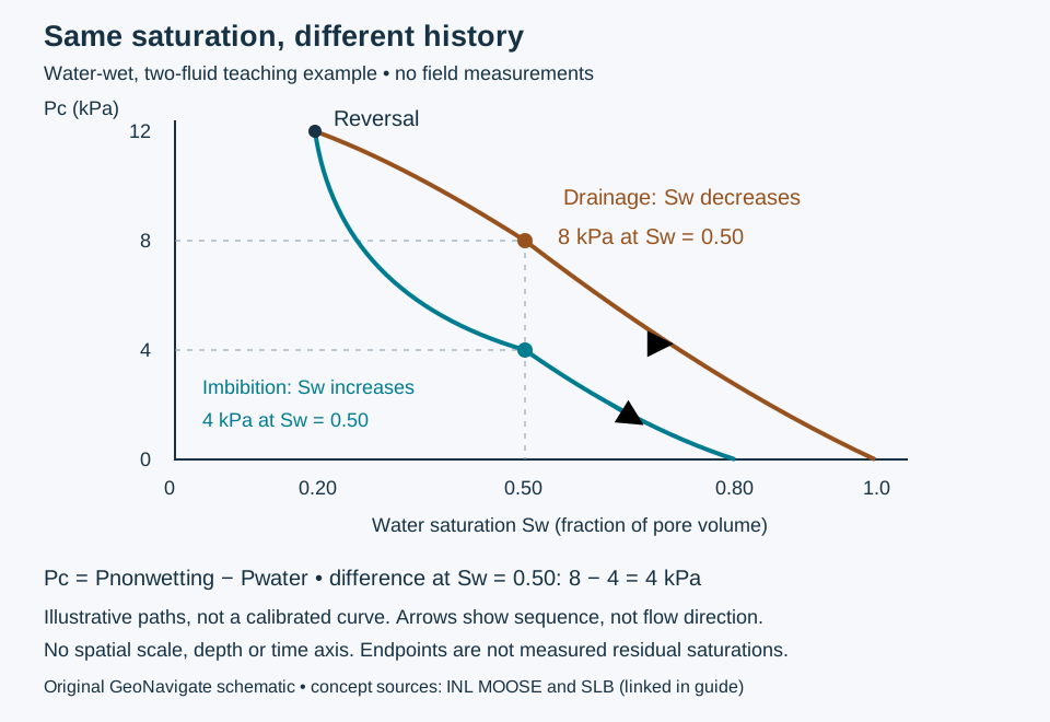
1. On the stipulated drainage path, Sw = 0.50 corresponds to Pc = 8 kPa.
2. After the reversal, the stipulated imbibition path passes Sw = 0.50 at Pc = 4 kPa.
3. The pressure-difference contrast is 8 − 4 = 4 kPa. Both states have 50% water-filled pore volume, but they do not have the same displacement history.

This is capillary-pressure hysteresis. A saturation-only lookup that ignores history cannot distinguish these two stipulated states. Neither value is a reservoir’s absolute pressure or a drilling margin. The plot does not provide a relative-permeability curve, a fluid velocity or a residual-saturation measurement.

Change the history, then reassess the comparison

If drainage reverses earlier, at Sw = 0.65, the illustrated return path is no longer the specified experiment. Do not interpolate a replacement from this drawing. Obtain appropriate measurements or a supported model with the new turning point. INL’s PorousFlow documentation explicitly retains reversal history when evaluating hysteretic curves.

Keep an interpretation record that can be checked

Record phase identities, wetting condition, initial saturation, displacement order, turning points, pressure convention and units beside a pressure–saturation result. Keep spontaneous uptake distinct from externally forced displacement. When comparing cores or model outputs, check whether the histories match before treating curve differences as a rock-quality difference.

A water-saturation estimate from logs supplies neither this history nor the applicable capillary curve by itself. Use core and fluid information to test the interpretation; do not turn the illustrative 4 kPa contrast into a field correction. This complements the Oilfield Glossary and the earlier throat-radius calculation, while answering a different question.

Sources and credit for this extension

• Idaho National Laboratory MOOSE: Hysteresis in PorousFlow — history-dependent curves and turning points.
• SLB: drainage and SLB: imbibition — phase-based terminology.

Compiled by GeoNavigate, checked 28 October 2026. Example values, explanation and SVG are original conceptual teaching material; no external expert review is claimed. Chaser Geological wellsite services · Contact.

One interface, two contact-angle conventions

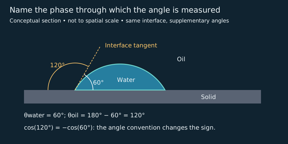
The contact angle includes the named fluid side. In this ideal flat-surface section, the solid baseline and interface tangent enclose 60° through water and 120° through oil. These are supplementary angles at the same contact, not two measurements of changed wettability.

Reconcile signs before comparing equations

Keep the earlier ideal tube at r = 10 μm and γ = 0.030 N/m, and stipulate water-wet conditions. With Pc = Poil − Pwater and θwater = 60°, the calculation is +2γ cos(60°)/r = +3 kPa. Using θoil = 120° requires the equivalent expression −2γ cos(120°)/r, also +3 kPa. Substituting 120° into the first expression without changing its angle convention instead produces −3 kPa: that is an inconsistent substitution, not evidence that the rock changed.

This conversion holds for the same ideal contact and fixed phase ordering. The drawing is a flat-surface angle construction, not the tube geometry used for the pressure calculation. A surface droplet alone supplies no throat radius. OpenPNM’s documented Washburn expression carries a leading minus sign; establish its phase and angle definitions before transferring inputs between software and hand calculations.

Preserve the measurement context

State the two fluids, solid, angle side and whether the contact line was advancing, receding or stationary. Roughness and displacement history can affect measured angles. Do not turn this one ideal angle into a whole-core wetting index, a recovery estimate or a drilling-pressure limit.

Sources checked 29 October 2026: SLB contact-angle definition and test context; OpenPNM Washburn model. Original geometry and calculation; no source artwork or field measurements reproduced. Compare oilfield contact angle, wettability and displacement history. Chaser services.

Input check: radius is half the diameter

A hypothetical image report gives throat diameter d = 10 μm. Convert it to radius r = d/2 = 5 μm before using Pc = 2γ cos θ/r. With the earlier water-wet convention, γ = 0.030 N/m and θ = 0°, the result is 12,000 Pa = 12 kPa. Entering 10 μm as radius would instead give 6 kPa, underestimating this ideal threshold by 50%. The lower panel of the shared schematic above records this separate case.

Equivalently, use Pc = 4γ cos θ/d with diameter in metres. Check the variable name, units, phase ordering and angle side before comparing hand calculations with software. OpenPNM documents a diameter input but writes its Washburn equation with radius; its leading minus sign also requires the angle-convention check above. An image-derived width is not automatically the controlling connected throat of a real rock. These invented values check input handling, not reservoir seal capacity.