Aquifer transmission and storage: worked examples

Two questions require two properties

How readily does an aquifer transmit water? How much water does it release when head changes? Transmissivity answers the first question. Storativity answers the second. Neither property alone gives a sustainable pumping rate. Geological boundaries, recharge, neighbouring users and discharge to streams also matter.

Transmission example: keep thickness and units explicit

Take an invented horizontal aquifer with uniform hydraulic conductivity K = 4 m/day and saturated thickness b = 25 m. T = Kb = 100 m²/day. This is a transmission property, not 100 cubic metres of stored water. For horizontal flow through layered material, sum each layer's K times thickness when the layers experience the same horizontal gradient. That sum is not the rule for vertical flow across the layers.

Storage example: a confined unit stays saturated

Use an independently assumed specific storage Ss = 0.000008 m⁻¹. Multiplying by b = 25 m gives S = 0.0002, dimensionless. Suppose hydraulic head falls uniformly by 2 m over a plan area A = 10,000 m², while both initial and final piezometric levels remain above the aquifer roof. The released storage volume is S A Δh = 0.0002 × 10,000 × 2 = 4 m³. Here Δh is a positive decline magnitude. Head change is not the thickness of a drained layer.

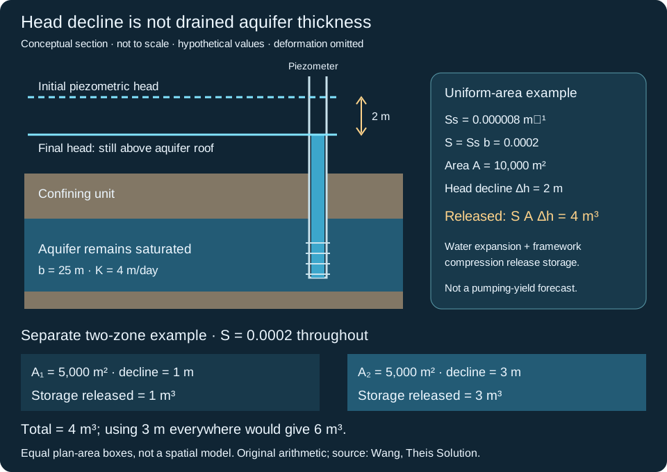
Why water is released without draining the pores

Lower pore pressure allows water to expand and can increase effective stress on the solid framework, reducing pore volume. Specific storage summarizes the resulting volume response per unit head change and bulk volume under the assumed mechanical conditions. It is not porosity: most pore water remains in place during a small pressure decline.

Contrast an unconfined water table

For a separate invented unconfined aquifer with specific yield Sy = 0.15, the same area and a 2 m water-table decline would release approximately Sy A Δh = 3,000 m³ by gravity drainage after sufficient drainage time. Elastic storage adds a smaller contribution in many such settings. This comparison uses different hypothetical materials and mechanisms; it is not a prediction that converting a confined aquifer will produce that amount. Its saturated thickness and therefore transmissivity may also change as the water table falls.

Worked example: where does the pore water go?

Consider a hypothetical rigid sample with bulk volume 1.00 m³ and porosity n = 0.30. Assume all pores are initially filled with water, none are isolated, and no water evaporates. Initial pore water is therefore 0.30 m³, or 300 litres. After gravity drainage reaches a specified endpoint, a collector contains 0.18 m³ (180 litres), leaving 0.12 m³ (120 litres) in the sample.

Specific yield is 0.18 ÷ 1.00 = 0.18 (18% of bulk volume). Specific retention is 0.12 ÷ 1.00 = 0.12 (12%). The balance is n = Sy + Sr = 0.30. Dividing 180 by 300 gives 60% of the initial water drained; that is a different denominator and is not the specific yield.

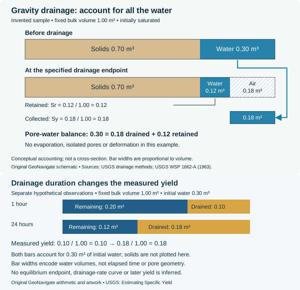
Specify the endpoint and the porosity convention

If only 0.10 m³ has emerged at an earlier observation, the collected fraction is then 0.10; do not silently label it the final Sy = 0.18. Drainage can continue slowly, especially in fine sediment. Report elapsed time, initial saturation and drainage boundary conditions. USGS column experiments also examined packing and wetting methods, illustrating why two tests need comparable preparation.

The simple balance above uses fully accessible initial pores. The Groundwater Project describes this balance using interconnected effective porosity. Effective porosity has application-dependent conventions, including petrophysical exclusions for bound water. Do not insert a log-derived value into a drainage balance without reconciling the definitions. Neither the retained nor drained fraction describes pore shapes, and neither is a sustainable well yield.

Saturated pores can lie above the water table

The water table is a pressure boundary, not necessarily the highest water-filled pore. The capillary fringe holds water above it at sub-atmospheric pressure. Smaller effective openings generally support greater rise. Its top varies with material and wetting history; the flat boundary below is a teaching simplification.

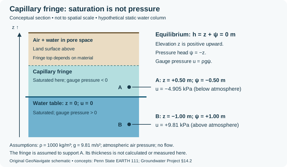
Worked pressure check at equilibrium

Choose the water table as elevation z = 0 m and let z increase upward. For this hypothetical static, constant-density water column, total hydraulic head h = z + ψ = 0 m, so pressure head ψ = −z. At A, 0.50 m above the table within the assumed capillary fringe, ψ = −0.50 m. At B, 1.00 m below, ψ = +1.00 m. With density ρ = 1000 kg/m³ and g = 9.81 m/s², gauge water pressure u = ρgψ gives −4.905 kPa at A and +9.81 kPa at B.

Both points have the same total head, so this static example has no hydraulic gradient driving flow. Negative gauge pressure means below atmospheric pressure, not a negative absolute pressure. The assumed fringe must be capable of supporting A; the calculation does not determine its thickness. During infiltration, evaporation or pumping, the hydrostatic relation may not apply.

Describe the boundary you actually observed

A wet core or moisture sensor alone does not identify zero gauge pressure. USGS recommends shallow-well water-level measurements for locating the water table; check the screen connection and stabilization before interpreting a level. Keep a confined-unit piezometric level separate. The vadose zone is often called unsaturated, although pressure-based usage includes saturated capillary water. State that convention in the log and distinguish a moisture transition from a measured water level.

Use the example as a balance, not a pumping forecast

A real drawdown cone is spatially variable. With constant S, integrate S times local head decline over the affected area rather than applying the maximum decline everywhere. Pumped volume need not equal storage loss because recharge, boundary inflow and reduced natural discharge may contribute. Delayed drainage, leakage and wellbore storage can change pumping-test interpretation. Record screen interval, datum, elapsed time and the conceptual aquifer model before comparing fitted parameters.

Worked example: weight drawdown by area

Consider a separate, invented two-zone approximation with S = 0.0002 throughout. Each zone covers 5,000 m²; declines are 1 m and 3 m. Storage releases are 0.0002 × 5,000 × 1 = 1 m³ and 0.0002 × 5,000 × 3 = 3 m³, totalling 4 m³. The lower panel of the shared figure shows the two equal plan areas.

The area-weighted mean decline is (5,000 × 1 + 5,000 × 3)/10,000 = 2 m. Applying the maximum 3 m everywhere instead gives 6 m³, an overestimate of 2 m³ or 50% relative to the calculated 4 m³. An unweighted mean works here only because the areas are equal. If S varies too, calculate each local product before summing. The zones are a stipulated approximation, not an observed drawdown map; keep both heads above the aquifer roof and treat storage release separately from total pumping.

Volume normalization follows Wang’s Theis Solution discussion, read 30 October 2026. The two-zone values and comparison are original. See storativity and its oilfield counterpart.

Sources and related learning

• USGS: estimating specific yield — operational volume balance and time dependence.
• Johnson, Prill and Morris (1963), USGS Water-Supply Paper 1662-A — column-drainage methods; DOI 10.3133/wsp1662A.
• The Groundwater Project: yield, retention and effective porosity — definition conventions and material context.
• Woessner and Poeter: aquifer and confining-unit properties — transmission, confined storage and gravity drainage.
• Wang: groundwater storage and the Theis definition — specific storage, units and volume normalization.
• Hydraulic testing: estimating storage properties — mechanical context and limitations.

Original teaching examples prepared 25 October 2026; no field measurements or expert review claimed. Read the Darcy-flow guide, effective-stress example, or Oilfield Glossary. For geological support, visit Chaser services or contact GeoNavigate.

Worked example: specific yield needs a drainage duration

A collected water volume is an observation at a stated time, not automatically the ultimate gravity-drainage yield. The USGS explanation of specific yield notes that drainage can take a long time, particularly in fine-grained material. Record elapsed time, sample dimensions, initial saturation and the drainage boundary conditions with the result.

Consider a separate invented test on 1.00 m³ of material containing 0.30 m³ of water initially. Assume fixed bulk and solid volumes, full initial saturation, no evaporation, no inflow and complete collection of discharged water. At 1 hour the collector contains 0.10 m³; at 24 hours its cumulative total is 0.18 m³. These are cumulative volumes, not rates.

1. At 1 hour, measured yield is 0.10/1.00 = 0.10. Remaining water is 0.30 − 0.10 = 0.20 m³.
2. At 24 hours, measured yield is 0.18/1.00 = 0.18. Remaining water is 0.12 m³.
3. During the intervening 23 hours, an additional 0.08 m³ drains. Its interval-average discharge is 0.08/23 = 0.00348 m³/h; that is not an instantaneous rate or a specific yield.

Do not call the water still present at one hour permanent specific retention, or assume the 24-hour result is equilibrium. The observations do not specify what drains later. The bulk-volume denominator is unchanged, so measured specific yield increases while the remaining-water fraction decreases. This illustrates why laboratory durations and drainage boundaries must be compared before transferring a value into an aquifer interpretation.

USGS methods source checked 31 October 2026; original arithmetic and artwork, no private measurements. Compare the oilfield entry and the earlier endpoint volume balance. For geological support, see Chaser Geological services or contact Chaser.

Worked example: equal diffusivity, different drawdown

Two aquifers can share hydraulic diffusivity without sharing drawdown magnitude. This comparison isolates the distinction using the ideal confined Theis model. It does not fit field measurements.

Hold the observation conditions fixed

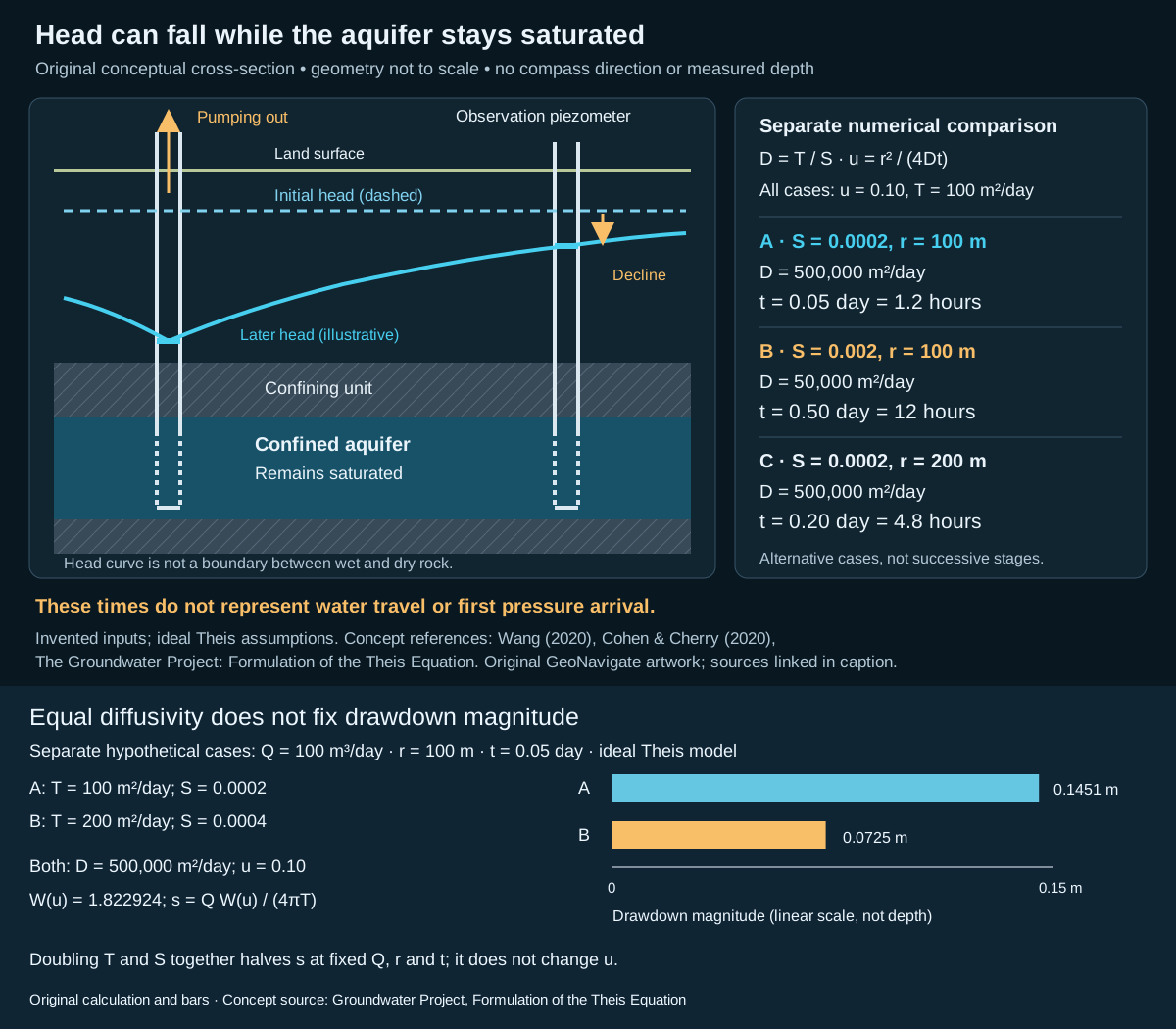
For both invented cases, set constant pumping rate Q = 100 m³/day, observation radius r = 100 m and elapsed time t = 0.05 day (1.2 hours). Case A has T = 100 m²/day and S = 0.0002; case B has T = 200 m²/day and S = 0.0004. Both give D = T/S = 500,000 m²/day, so u = r²/(4Dt) = 0.10 in each.

Evaluate the well function W(u) = ∫ᵤ∞ exp(−x)/x dx: W(0.10) ≈ 1.822924. Using s = Q W(u)/(4πT), case A gives 0.145064 m and case B gives 0.072532 m. Rounded display values are 0.1451 m and 0.0725 m. The exact ratio within these model inputs is one half: the shared W cancels and T doubles.

The expanded head-response schematic shows both results with a common linear drawdown scale. Its earlier conceptual cross-section is not a computed profile for these numerical cases.

What the comparison does and does not establish

Use the same homogeneous, isotropic, laterally infinite confined model for both cases: full penetration, negligible well radius, instantaneous elastic storage, no leakage and initially uniform head. The units remain saturated. Changing those assumptions can change the result. Equal diffusivity is therefore insufficient to predict amplitude: retain pumping rate and transmissivity as separate inputs.

If case B instead pumps at 200 m³/day, Q/T also matches case A and the calculated drawdowns match. Neither comparison supplies a contaminant travel time or a sustainable pumping rate. See Oilfield Glossary context.

Reference checked 31 October 2026: Woessner, Stringer and Poeter (2023), Theis formulation, equations 25–26. Numbers and expanded artwork are original. Chaser Geological services.

Worked example: thickness-weighted confined storage

Start with the definition of specific storage: released water volume per bulk volume per unit head decline. The following is an original accounting exercise, not a pumping-test solution.

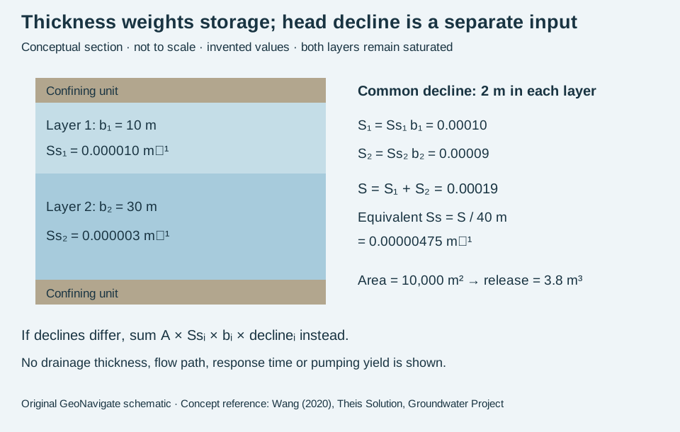
Sum the layer contributions

Assume a confined column has a 10 m layer with Ss = 0.000010 m⁻¹ and a 30 m layer with Ss = 0.000003 m⁻¹. Both stay saturated, the storage coefficients remain constant under the specified mechanical conditions, and each layer experiences the same 2 m head decline over 10,000 m².

Layer contributions to storativity are 0.000010 × 10 = 0.00010 and 0.000003 × 30 = 0.00009. Their sum is 0.00019. The column-equivalent specific storage is 0.00019 / 40 = 0.00000475 m⁻¹. Released volume is 10,000 × 0.00019 × 2 = 3.8 m³, also obtained as 2.0 + 1.8 m³ from the separate layers.

Test two tempting shortcuts

An unweighted mean of the two Ss values is 0.0000065 m⁻¹. Multiplying that by 40 m, area and decline gives 5.2 m³, overstating this example by 1.4 m³ because the layers have unequal thicknesses.

Now change only the declines: layer 1 declines 1 m and layer 2 declines 3 m. Separate accounting gives 10,000 × (0.00010 × 1 + 0.00009 × 3) = 3.7 m³. A common 2 m decline would give 3.8 m³ and is no longer the stated model. Determining actual layer heads requires flow, boundary and time information; storage arithmetic alone cannot supply them.

Concept reference checked 31 October 2026: Herbert F. Wang (2020), Theis Solution, equations and volume normalization. Numbers and illustration are original. Compare wellsite terminology; contact Chaser Geological services for geological support.

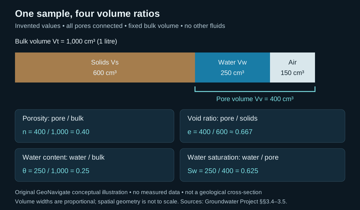
One sample, four different volume ratios

A moisture reading and a porosity estimate are not interchangeable. Void ratio uses solid volume as its denominator; volumetric water content uses whole-sample volume. Water saturation uses pore volume. Specify the volume convention before comparing core descriptions, soil measurements or logs.

Worked example: audit the denominators

Invent a 1,000 cm³ sample containing 600 cm³ of solids, 250 cm³ of water and 150 cm³ of air. Assume all pores are connected, no other fluid phases occur and the bulk volume stays fixed. Pore volume is 250 + 150 = 400 cm³; the three components sum to the bulk volume.

• Porosity n = 400/1,000 = 0.40 (40%).
• Void ratio e = 400/600 = 2/3 ≈ 0.667. Check n = e/(1 + e) = 0.40.
• Volumetric water content θ = 250/1,000 = 0.25 (25%).
• Water saturation Sw = 250/400 = 0.625 (62.5%). Check θ = n Sw = 0.40 × 0.625 = 0.25.

Change water occupancy without changing pore space

In a second invented state, 100 cm³ of water leaves and an equal air volume enters without deformation or evaporation. Water content becomes 150/1,000 = 0.15; saturation becomes 150/400 = 0.375. Porosity and void ratio remain unchanged. This imposed volume transfer alone does not establish specific yield: no gravity-drainage endpoint or test duration was specified.

What the arithmetic cannot tell you

The volume bar says nothing about pore throats, connectivity, permeability or flow direction. Real samples can contain isolated pores, shrink during drying or swell when wetted. Match total versus effective pore conventions across the inputs; the all-connected assumption makes them identical only in this example. A gravimetric water content is a mass ratio and requires density information for conversion. Do not infer the water table or a capillary-pressure curve from one moisture value.

Original explanation and invented arithmetic checked 26 October 2026; no expert review claimed. Continue to the Oilfield Glossary, geology guides, Chaser Geological services or contact GeoNavigate.

Head response is not groundwater travel time

A pumping well can change the level in an observation well without draining the rock between them. A potentiometric surface describes head in a specified unit. In a confined aquifer, a falling level above the roof records declining pressure while the aquifer remains saturated. It is not a newly exposed water table inside that unit.

Worked example: compare the same dimensionless response coordinate

Use the earlier invented confined-aquifer values T = 100 m²/day and S = 0.0002. Their ratio, hydraulic diffusivity, is D = T/S = 500,000 m²/day. This is an area divided by time, not metres per day. The equivalent ratio K/Ss gives the same result for the uniform thickness assumed above.

For the ideal Theis model, u = r²S/(4Tt) = r²/(4Dt). Choose u = 0.10 only as a comparison coordinate; it is neither a first-arrival threshold nor a measured drawdown. At radial distance r = 100 m, rearrangement gives t = 100²/(4 × 500,000 × 0.10) = 0.05 day = 1.2 hours.

1. Keep T fixed and increase S tenfold to 0.002: D becomes 50,000 m²/day, and the same u at 100 m occurs at 0.50 day = 12 hours.
2. Return to the original T and S, but double r to 200 m: t becomes 0.20 day = 4.8 hours. The factor of four follows from squared distance, not a constant propagation speed.

These are alternative model comparisons. To calculate drawdown magnitude, supply pumping rate Q and evaluate s = Q W(u)/(4πT), where W is the Theis well function. Equal u alone does not imply equal drawdown if Q/T differs. Nothing here predicts when a water molecule or dissolved contaminant reaches the well.

Match the model to the geological setting

This exercise assumes a laterally infinite, homogeneous, isotropic confined aquifer, constant T and S, a fully penetrating well of negligible diameter, constant-rate pumping and instantaneous elastic storage response. It omits leakage, recharge boundaries, wellbore storage and partial penetration. A real response can depart from this model; the arithmetic is not a field calibration or a recommended test duration.

Keep the measurements traceable

• Record observation time, screen interval and a common elevation datum. A well open across several units can mix their responses.
• Distinguish drawdown from a change in saturated thickness. Check whether head has fallen below the confined-unit roof before continuing to use a constant-thickness model.
• Describe pressure communication separately from transport. Use the Darcy and pore-water velocity example for the latter, with its own assumptions.

References and scope

• Wang (2020), Diffusion Equation — diffusivity and transient head redistribution.
• The Groundwater Project, Formulation of the Theis Equation — model assumptions, u and the well function.
• Cohen and Cherry (2020), confined-aquifer head — potentiometric representation.
• Mower (1973), USGS IMAP 766-L — published potentiometric-map example; publisher-indexed abstract checked.

Sources checked 27 October 2026. Original explanations, arithmetic and artwork; no private well data or external expert-review claim. Continue to the Oilfield Glossary, Geology Guides, Chaser Geological services or contact Chaser Geological.

Artesian does not always mean a flowing well

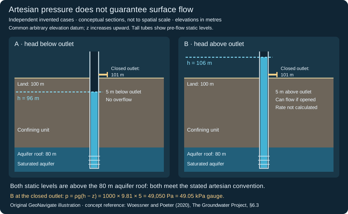
Artesian condition describes confined water that rises above the aquifer roof in a connected well. Flow at the surface requires a further comparison: is the undisturbed head above the available outlet? A potentiometric surface is a representation of head, not a rock contact or the top of saturated pores.

Worked example: compare three elevations

Assume a fully saturated confined aquifer has roof elevation 80 m, land elevation 100 m and a possible discharge outlet at 101 m. Consider two independent static-head cases for constant-density freshwater, with the observation tube connected only to that aquifer.

• Case A: h = 96 m. The level is 16 m above the roof, so this meets the stated artesian convention. It is 5 m below the outlet and 4 m below land. The well will not overflow that outlet under these conditions.
• Case B: h = 106 m. The level is 26 m above the roof and 5 m above the outlet. A sufficiently tall tube could hold this static column. Opening the lower outlet provides potential for discharge; the drawn 106 m level is the pre-flow measurement, not a promise that head remains fixed during flow.

Translate head into a static pressure difference

With elevation z positive upward, h = z + p/(ρg) when velocity head is negligible. For Case B at the closed outlet elevation, pressure head is h − z = 106 − 101 = 5 m. Taking ρ = 1000 kg/m³ and g = 9.81 m/s² gives gauge pressure p = 1000 × 9.81 × 5 = 49,050 Pa = 49.05 kPa. Gauge pressure is relative to the local atmosphere. This calculation assumes the outlet communicates with a continuous static water column.

Do not apply that submerged-point calculation at Case A's dry outlet: its equilibrium water surface is lower. At an open free-discharge outlet in Case B, pressure approaches atmospheric while energy is spent in flow and losses. Predicting rate requires aquifer transmission, well geometry, outlet restrictions and boundary conditions. The 5 m excess head alone is not a flow-rate estimate.

Record what the observation supports

Use a common elevation datum and identify screen interval, fluid density, measurement time and whether a reading was static or flowing. An open interval spanning multiple units can mix their heads. The words “artesian” and “flowing” are sometimes used differently; report the measured elevations as well as the label. This is an educational groundwater example, not a well-control design or an inference about hydrocarbon reservoir pressure.

Concept reference read 29 October 2026: Woessner and Poeter (2020), section 6.3. Pressure-head reference: The Groundwater Project, review of hydraulic head (primary-source indexed text checked). Arithmetic, hypothetical observations and artwork are original; no measured well data or external expert review claimed. Continue to artesian conditions in the Oilfield Glossary, the groundwater-flow guide, Chaser Geological services or contact Chaser Geological.